27. AC Drives#
This would be the last lecture of this course. We will have a brief introduction to how the ac machines can be controlled. After taking this lecture, we should be to able to understand the basic architecture of variable speed AC drives, tell the operation principle of single phase and three phase ac inverters, and do relevant calculations.
27.1. Drive system recap#

Let us first have a recap of the drive system.
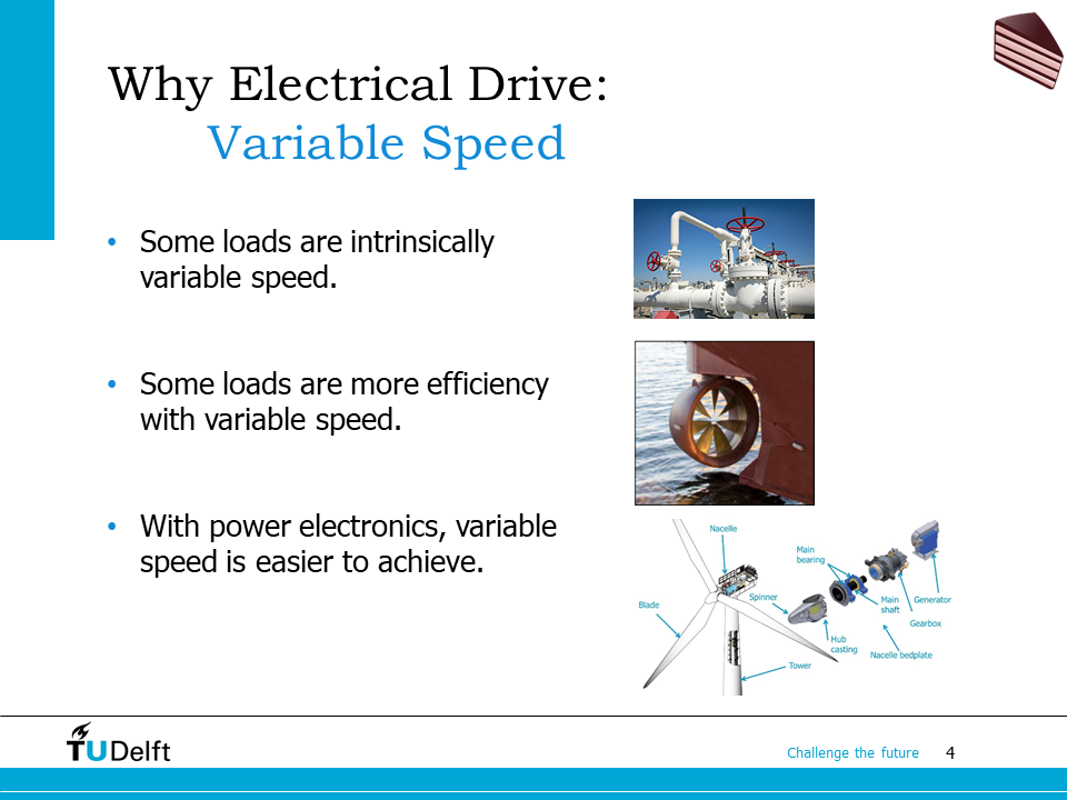
We know from the DC drive part of the course that, a drive system is often needed in various applications, mainly because by varying the speed with drives, the system efficiency can be improved, or the size of the mechanical system will be reduced. By using power electronics, it is easier to vary speed with various types of electrical machines.
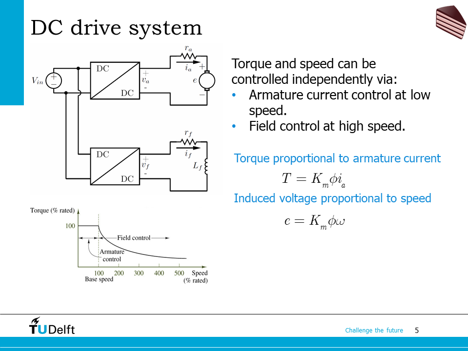
In the DC drive system, we have learned that by using two DC-DC converters, the field (flux per pole \(\phi\)) and the armature current can be controlled independently. By keeping \(\phi\) at rated value and controlling the armature current \(I_a\) at low speed, and field weakening (reducing \(\phi\) to limit \(e\)) at higher speed, we are able to achieve the torque-speed characteristic shown on the bottom.
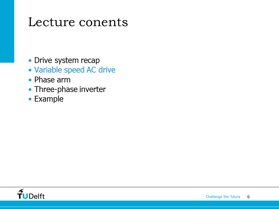
27.2. Variable speed AC drives#
The operation principle of the AC drive system is similar to the DC drive system, as we will see in the following slides.
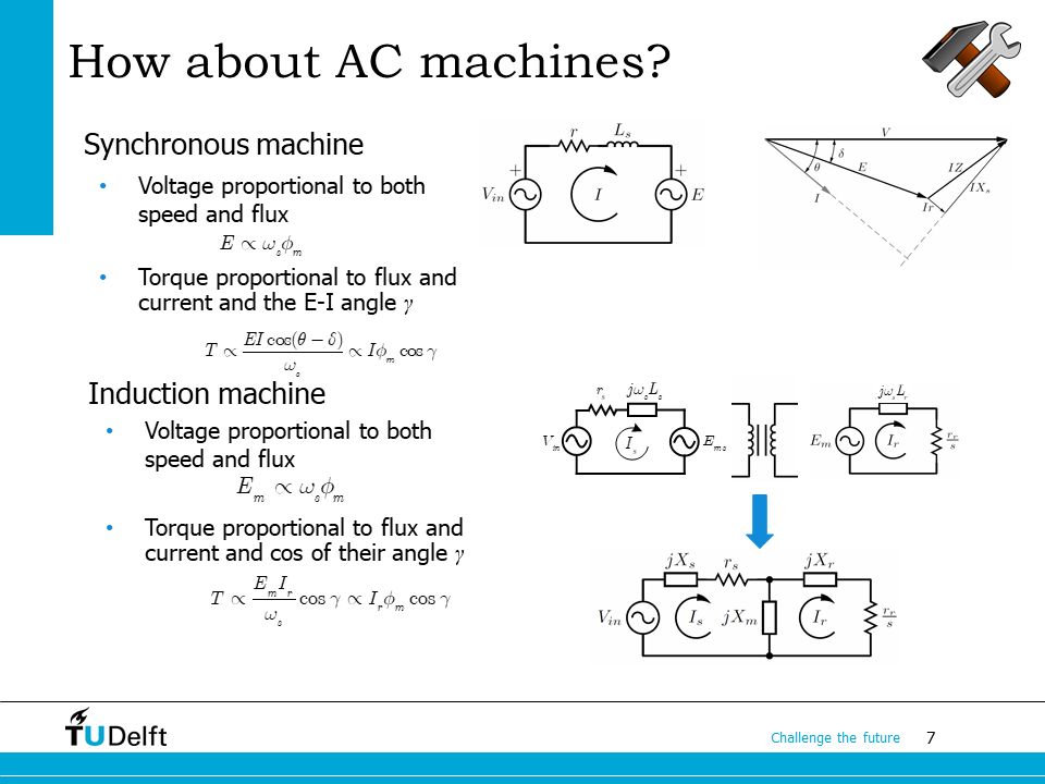
First, let us check the synchronous machine. Similar to the DC machine, we know the induced voltage is proportional to both the flux per pole and the speed. From the developed power, we are able to see that the torque is proportional to the flux per pole, the armature current, and also the angle \(\gamma\) between the induced voltage and the armature current.
Similarly, for the induction machine, the induced voltage is also proportional to both the flux per pole and the speed. Dividing the air gap power by the synchronous speed, we will see that the torque is also proportional to the flux per pole, the armature current, and also the angle \(\gamma\) between the induced voltage and the armature current.
Therefore, for both types of AC machines, the induced voltages are dependent on the speed and the flux; while the torque is determined by the flux and the armature current, which is similar to the DC drive. The only difference is a difference that, in AC machines, we also have to deal with the angle between the induced voltage and the armature current \(\gamma\).
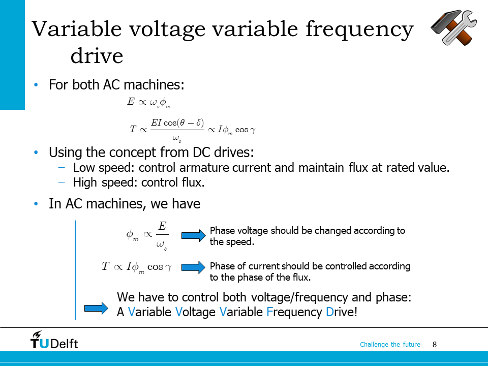
Therefore it is possible to control the AC drive using the concept from DC drives: we can maintain the flux at rated value and control the armature current at low speed, and do field weakening at high speed.
Since the induced voltage is changing as a function of the rotating speed, and the electrical frequency also changes as synchronous speed changes, to efficiently control the torque of the ac machine, we have to control the voltage, frequency and the phase of current together. Therefore, the AC drive is also called the Variable Voltage Variable Frequency Drive (VVVFD).
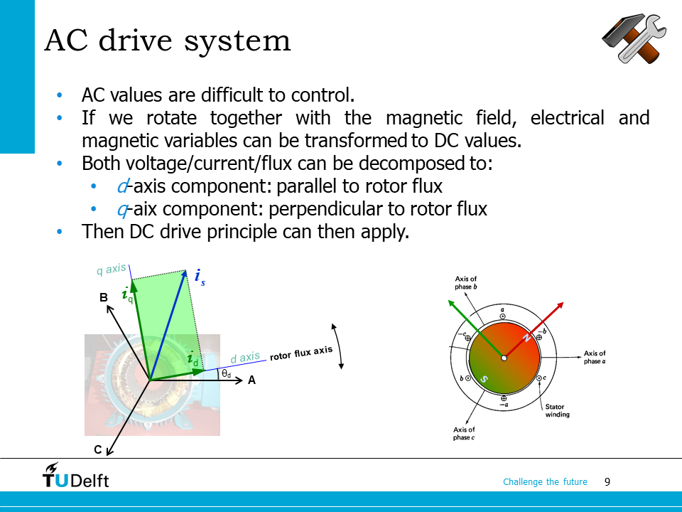
However, compared to a DC drive, AC voltages are difficult to be regulated by a controller directly. Fortunately, because of the symmetry of the three phases, we are able to use transformation to transform the three phase AC quantities to DC quantities. The principle is to express quantities including flux linkages, currents and voltages in a coordinate system which is rotating together with the magnetic field. Therefore, each quantity can be decomposed into two components: 1). d-axis component, which is in the direction of the rotor flux; 2). q-axis component, which is perpendicular to the rotor flux.
We can prove mathematically that by transformed balanced ac quantities into a coordinate system rotating at the synchronous speed, DC quantities will be obtained. As is shown in the script below.
from sympy import *
from IPython.display import display, Markdown, Math, Latex

t, theta, I_m, N, g, mu_0 = symbols('t, theta, I_m, N, g, mu_0')
omega = symbols('omega', positive=True)

# three phase, a-b-c sequence, hence rotate CCW

i_a = I_m*cos(omega*t+theta)
i_b = I_m*cos(omega*t - 2*pi/3+theta)
i_c = I_m*cos(omega*t + 2*pi/3+theta)

# define a rotating frame rotates at speed omega
i_a_d = i_a*cos(omega*t)
i_a_q = i_a*sin(omega*t)

i_b_d = i_b*cos(omega*t-2*pi/3)
i_b_q = i_b*sin(omega*t-2*pi/3)

i_c_d = i_c*cos(omega*t+2*pi/3)
i_c_q = i_c*sin(omega*t+2*pi/3)

# sum and multiply it by 2/3 to keep the amplitude unchanged
i_d = 2/3*(i_a_d+i_b_d+i_c_d)
i_q = 2/3*(i_a_q+i_b_q+i_c_q)
display(Math('$i_d =$'), i_d.simplify())
display(Math('$i_q =$'),i_q.simplify())
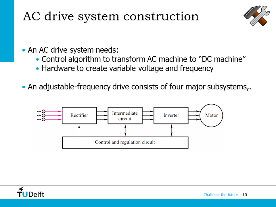
As we can see, to construct an AC drive system, both software and hardware are needed. Inside the software, we need the control algorithm to transform the AC machine to a virtual “DC machine”. For the hardware, we need the a power converter to convert from DC to AC, which is also called an “inverter”. The architecture of a typical AC drive system is shown on the bottom of the slide.
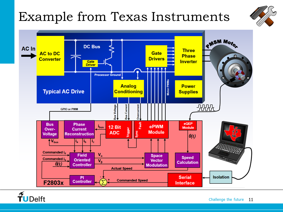
Here it shows a detailed hardware/software structure of an AC drive system based on the Texas Instrument platform. As you can see, encoders are used to measure the machine speed, and the ADCs are used for the current and voltage feedback. There is also algorithm running inside the digital processor for the transformation and control (field oriented controller) .
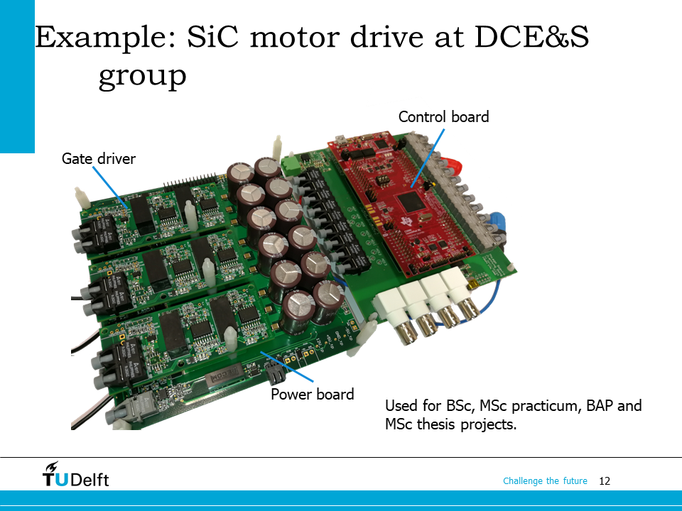
Here it shows an AC drive hardware developed at TU Delft using the latest Silicon Carbine MOSFET technology.
27.3. Phase arm#

Now let us study the construction of the inverter, which is the core part of the AC drive hardware. We first take a look at the basic building block, the phase arm.
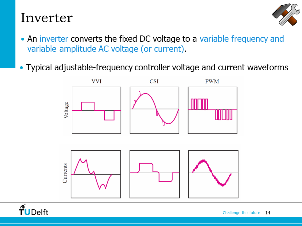
As the name indicates, an inverter converts the DC voltage to a variable frequency and variable amplitude AC voltage or current. Based on the operation principle and wave shapes involved, the inverter can be classified into the Variable Voltage inverter (VVI), current source inverter (CSI) and the pulse width modualted (PWM) voltage source inverter (VSI). In this lecture, we focus on the PWM VSI since it is the most commonly used one.
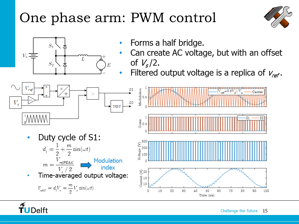
A phase arm is in essence a half bridge. If we modulate a half bridge using an AC modulation waveform, we will be able to obtain an AC output by taking the time-average of each switching cycle. Switching harmonics can be filtered out using inductance, therefore, we will observe more sinusoidal waveform from the current. As we can see, a phase arm is able to function as a single phase inverter, but its output has an offset of \(V_s/2\).
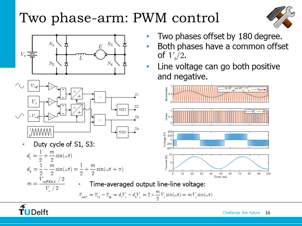
If we connect two phase arms in parallel and connect the load in between, a H-bridge is obtained. If use two reference waveforms with 180 out of phase to modulate the two phase arms, apparently, the two phase arms are able to produce two AC outputs with reversed polarities, but the same DC offset. The load voltage fundamental component, which is obtained from the voltage difference between the two phase legs, will be
where \(m\) is called the modulation index. Now compared to the single phase arm case, the DC offset is gone. When \(m=1\), maximum ac output amplitude is achieved, which is \(V_s\), when \(m=0\), output voltage would be 0.
27.4. Three phase inverter#
By putting three phase arms together, it is possible to have a three phase full bridge and use it as a three phase inverter.
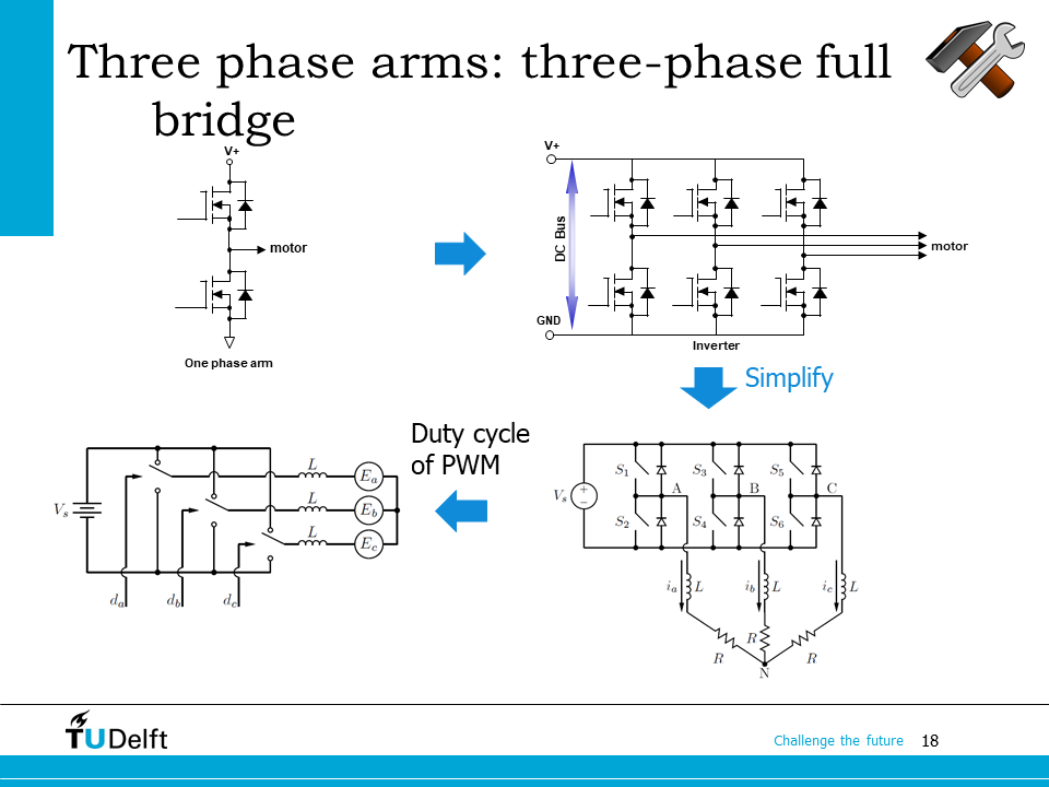
Each phase arm can be modulated to obtain a fundamental ac voltage with an offset.
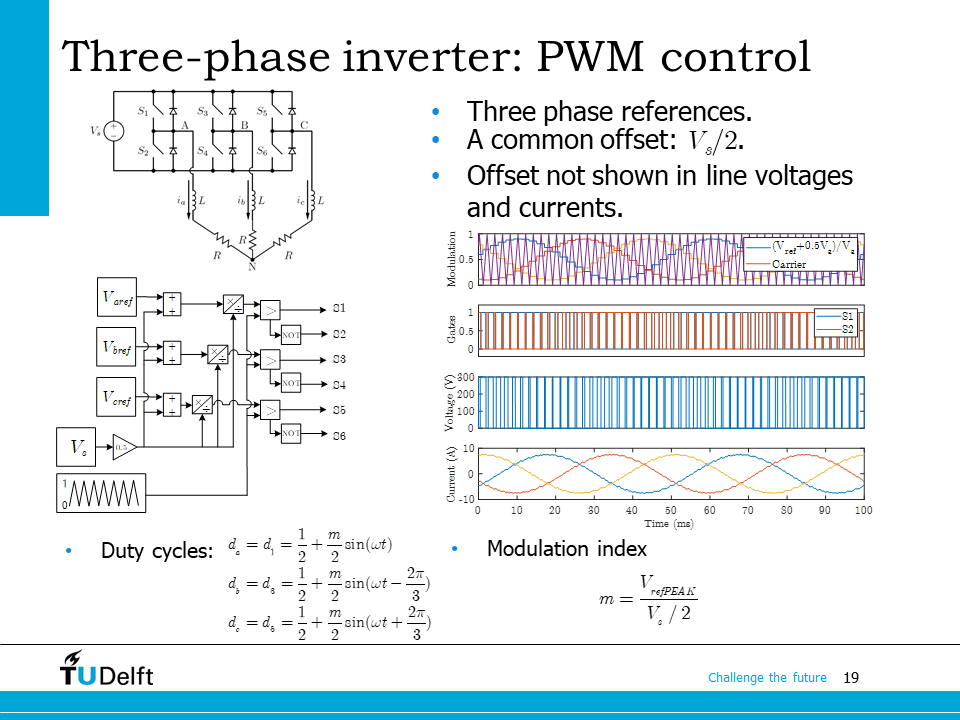
If all three phases are modulated with three phase symmetric references with a common DC offset, three phase AC outputs can be obtained. There are multiple ways to choose the common DC offset. The most straightforward way is to choose \(V_s/2\), as we did for the H bridge.
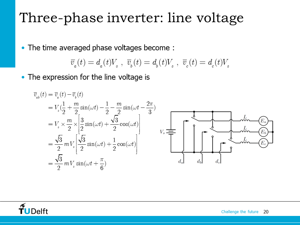
Since all three phase have the same DC offset, it is easy to calculate that, the DC offset is eliminated in the line-line voltages, as shown on the slide.
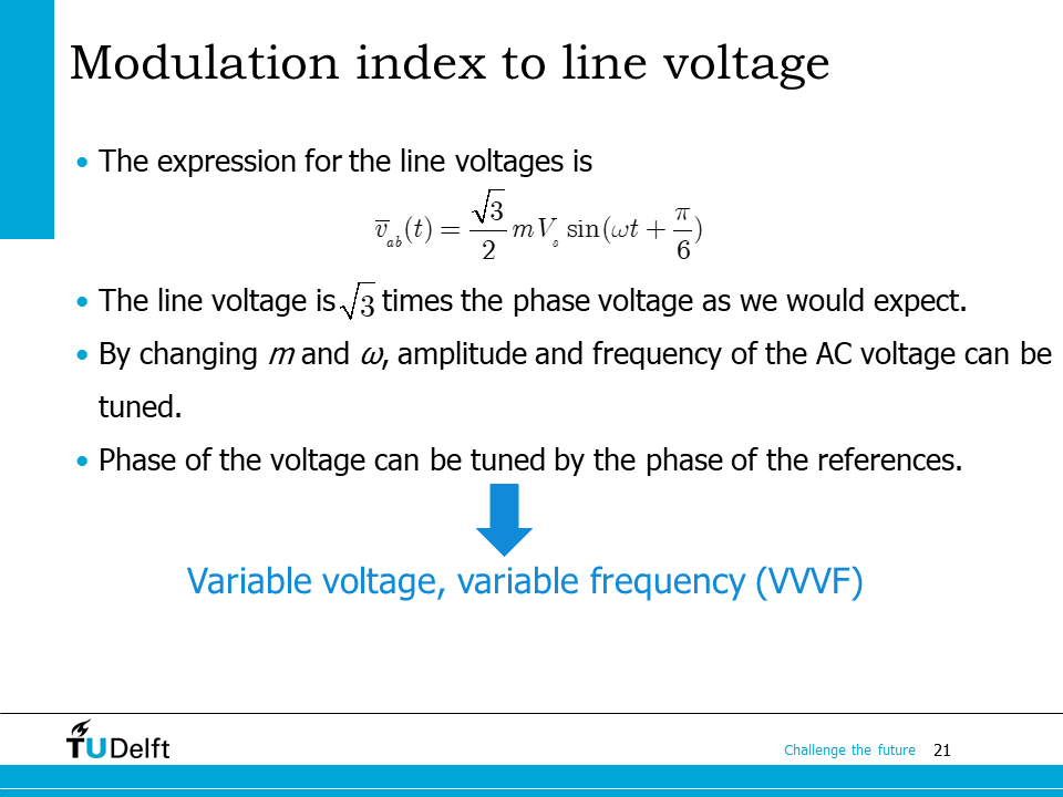
From the final line voltage expression, we can see that, in order to achieve the variable-voltage variable-frequency regulation, we should change the modulation index \(m\), the angular speed \(\omega\), and the phase angle of the reference for the modulation of the three phase inverters.
27.5. Example#

An example is used to practice the calculation for the three phase inverter.
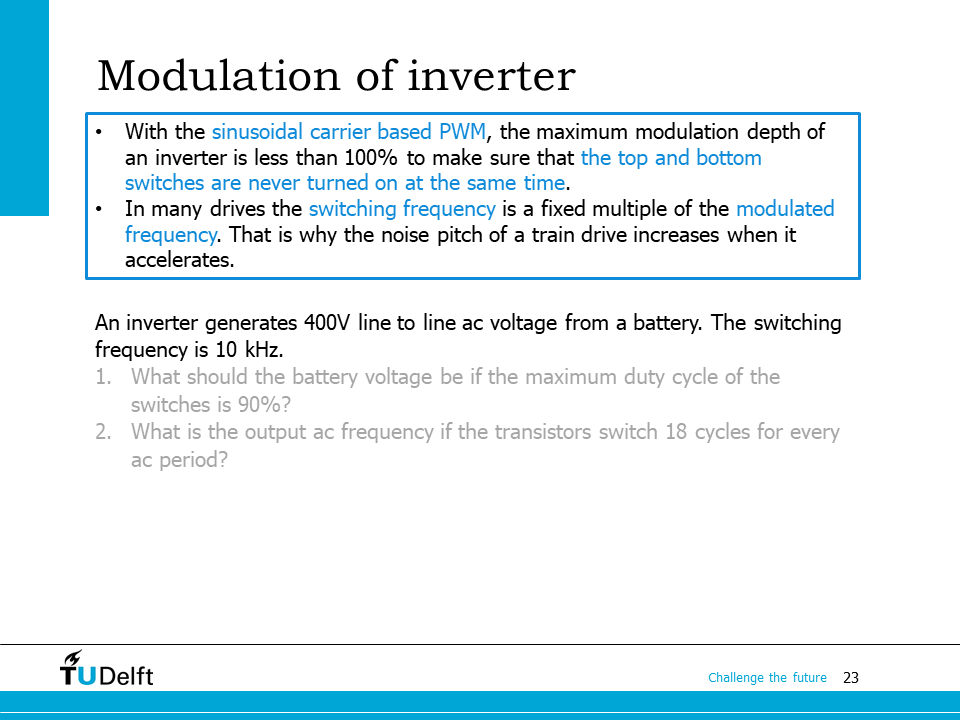
If the modulation index is \(m\), the maximum and minimal duty cycle would be \(m+0.5\) and \(0.5-m\).
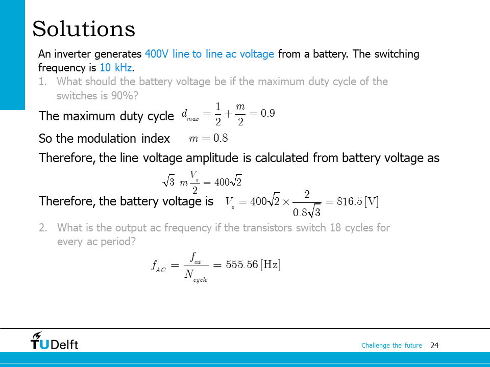
The solution is shown on this slide.