16. Transformer#
In the last lecture, the ideal transformer is studied. This lecture will introduce the non-ideal part of the transformer: leakages and loss, which will be reflected as leakage inductance and resistances.
After taking the lecture, we should be able to understand the practical construction of a transformer and apply the equivalent circuit model to solve transformer problems.
16.1. Practical transformers and applications#
We first start with various applications of transformers and how a transformer is made in practice.
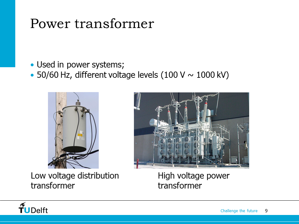
Transformers are all around us and come in many different shapes and sizes. In power grid we have distribution power transformer which operates at 400 V and 50 Hz in the Netherlands, as shown on the left. They are often mounted on poles, or sometimes in electrical rooms. You may have encountered them in your local community.
For the power transportation system, the power transformers used are much larger and have higher voltage ratings. What you see on the right hand side is a typical high voltage transformer operates in substations.
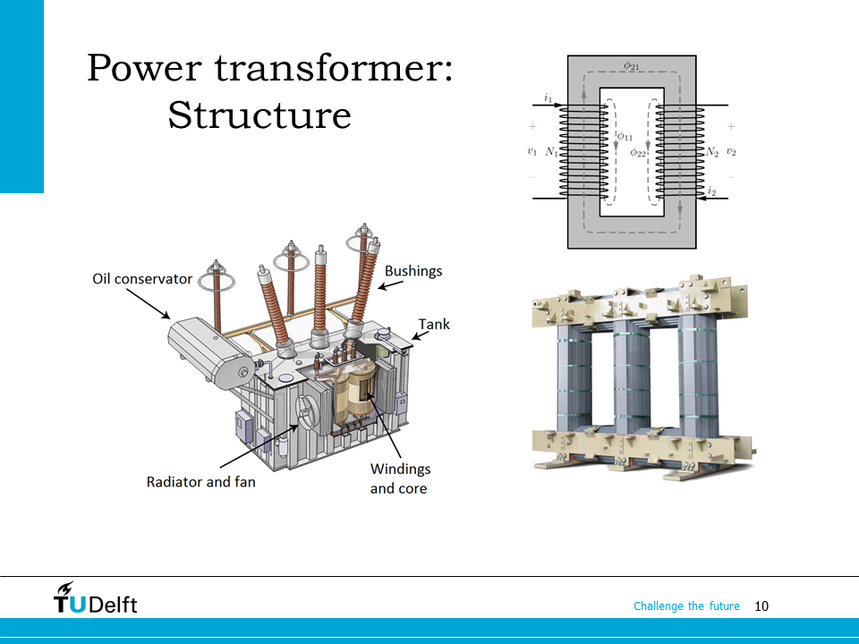
Top right is the ideal model of the transformer. Bottom left shows the structure of a real power transformer. The brown poles on the transformer are called bushings, which are hollow electrical insulators that allow the electrical conductors to pass safely through the grounded tank of the transformer. There are two sets of phase bushings: the larger ones are for high voltage windings, and the tiny ones are for low voltage windings. The bushings with concentric rings on the far side are surge arresters, which are able to absorb electrical transients to protect the transformer. The concentric rings on top of them are called corona rings, which is there to prevent corona discharge.
The three phase primary and secondary windings are wounded around magnetic cores made from silicon steel laminations, which is shown on the bottom right.
The magnetic core and windings are submerged in transformer oils enclosed by the tank. The transformer oil is used to insulate, suppress corona discharge and arcing, and to serve as a coolant. The conservator tank of transformer provides adequate space to the expansion of transformer oil when it is heated up by losses or ambient.
The radiators and fans installed on the tank are used to dissipate heat generated by winding and core losses inside the transformer.
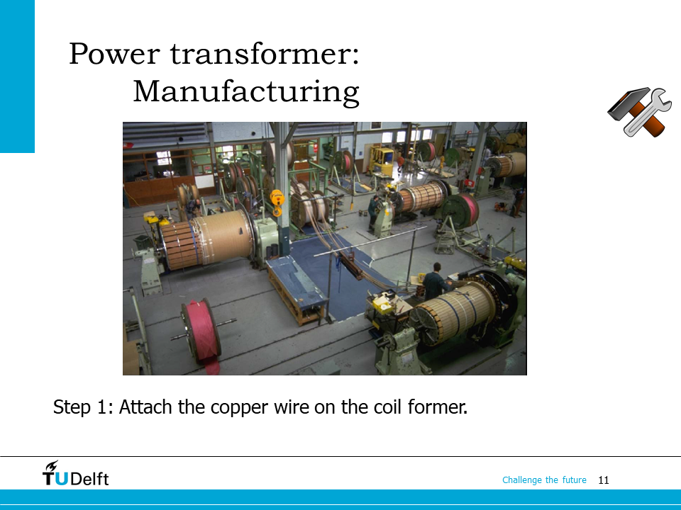
Here it shows the manufacturing process of a power transformer. The first step is to attach copper conductors to the coil former. Depending on the type of transformers, the coil may have a helical shape or a disk shape.
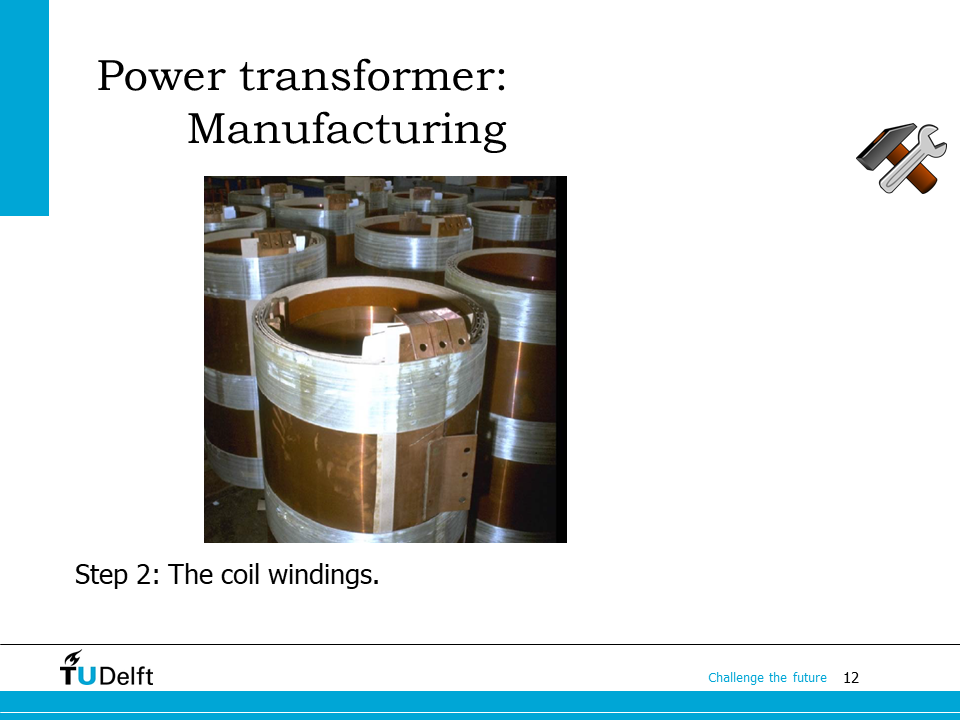
The copper conductors used are not necessarily to have round shapes. For example, flat copper condutors are used to construct the coil on this slide.

Then the silicon steel laminations are cut or punched into different widths to make the magnetic core.
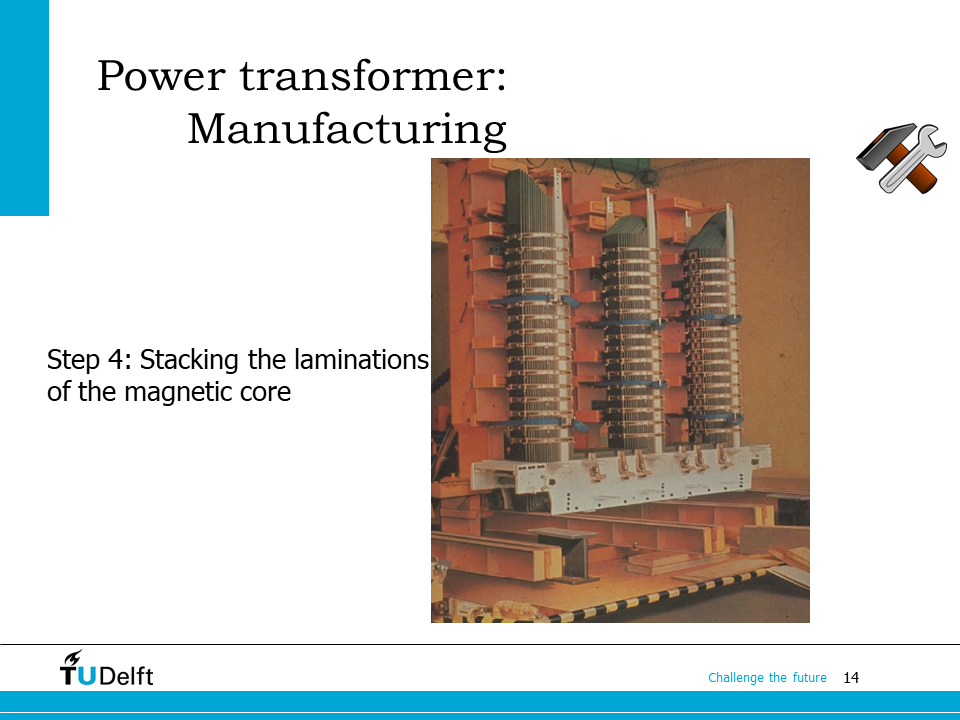
The punched laminations are then stacked together and fixed by mechanical structures to form the magnetic core.
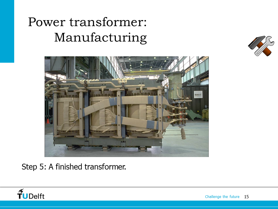
Then the coils will be mounted to the magnetic core to form the primary and secondary three phase windings, and extra insulation will be added so that the conductors are well insulated from the supporting structure and the magnetic core.
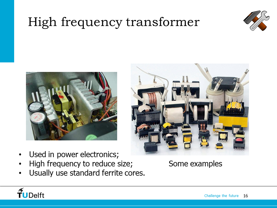
Transformers are also extensively used in power electronics. These transformers usually operate at high frequencies: from several kHz to MHz. High frequency is used because to convert the same power, a higher frequency helps reduce the size of transformer. For high frequency transformers, pre-made standard ferrite cores are used.
There are some examples as shown on the right hand side of the slide.
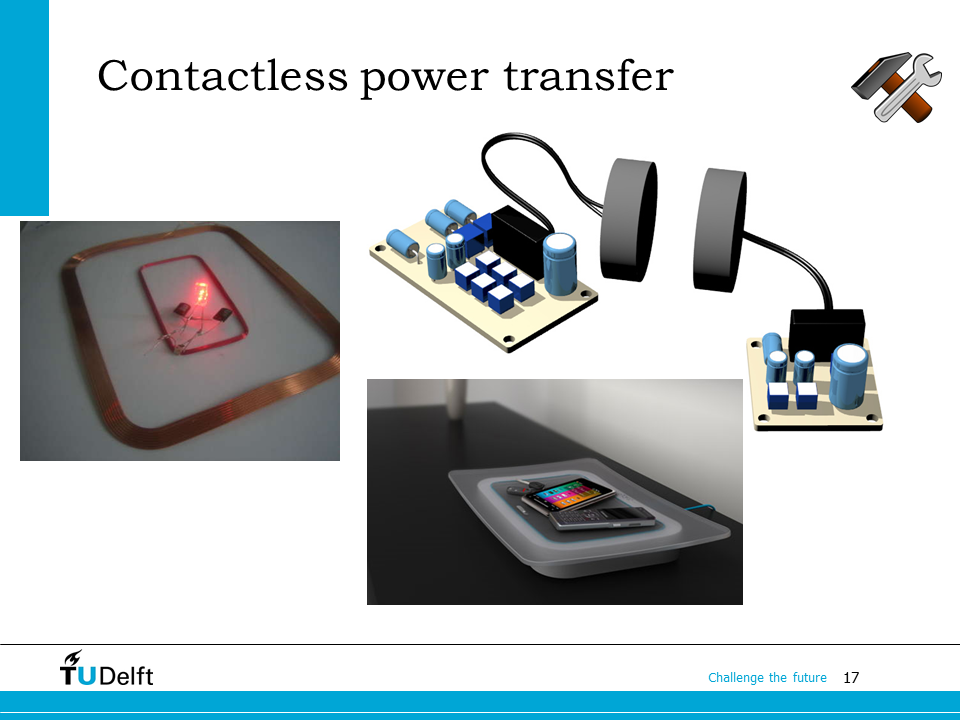
Transformer is also used for contactless power transfer. For these transformers, “air core” is used instead of ferromagnetic core, so the magnetic flux flows in air and is not regulated by the magnetic core. As a consequence of that, the coupling factor between the two coils is very low. To efficiently transfer power through the two loosely coupled coils, compensation capacitors are usually added to create a resonance power conversion. This will be further elaborated in the module 1 of the course lab.
16.2. Mutual inductances in transformers#
Let us now deal with the non-ideal behaviours of the transformer.
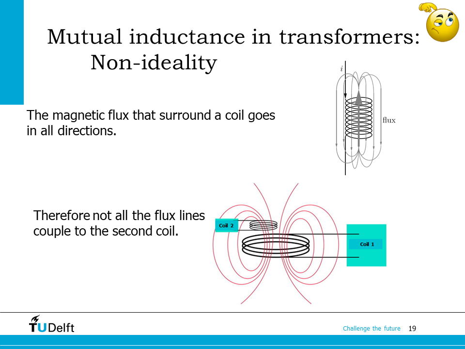
In practice, not all flux can be short-circuited by the magnetic core: there is always part of the flux flows to surroundings. Therefore, there would be part of the flux generated from one coil does not couple with the secondary coil.
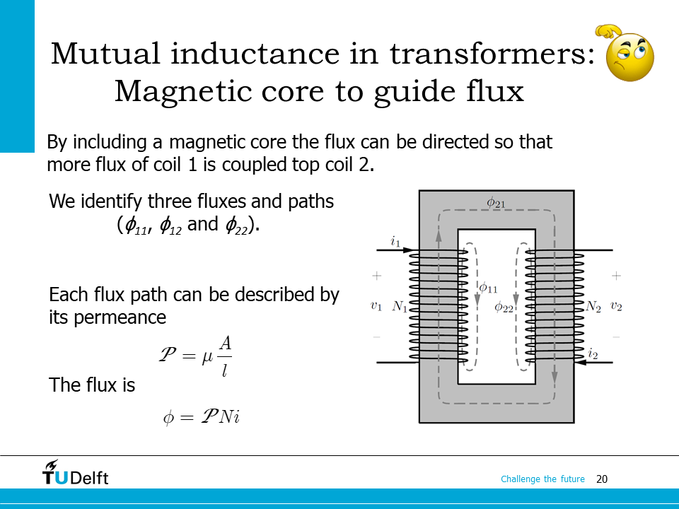
As we can see here, the flux lines can be divided into three paths:
\(\phi_{11}\): those are linked with coil 1 through surrounding air, but do not go to coil 2 through the magnetic core;
\(\phi_{12}\): those link both coil 1 and coil 2 through the magnetic core;
\(\phi_{22}\): those are linked with coil 2 through surrounding air, but do not go to coil 1 through the magnetic core.
For the three magnetic flux paths, we can define their permeance respectively: \(\mathcal{P}_{11}\), \(\mathcal{P}_{12}\) and \(\mathcal{P}_{22}\). If the total MMF given by the coils is \(Ni\), we have
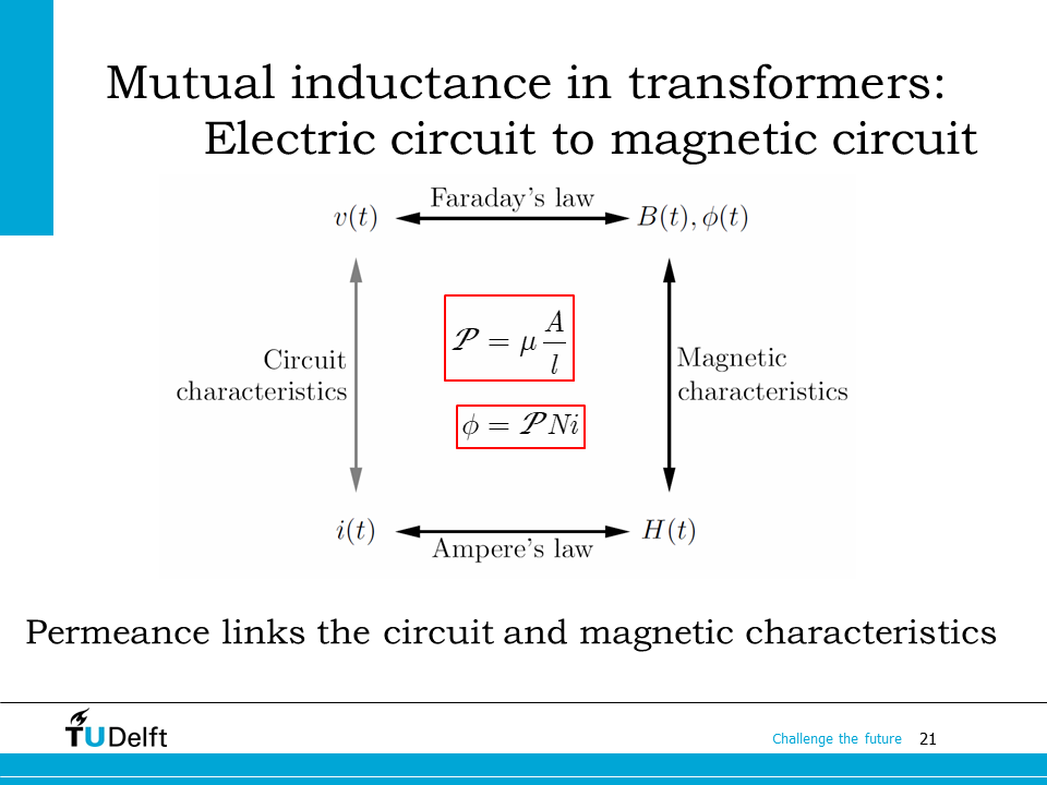
Here we used the magnetic principles we learnt in the last lecture, as shown in this flow chart. Let us continue to apply this flow chart to derive the inductances of the coils based on the permeance.
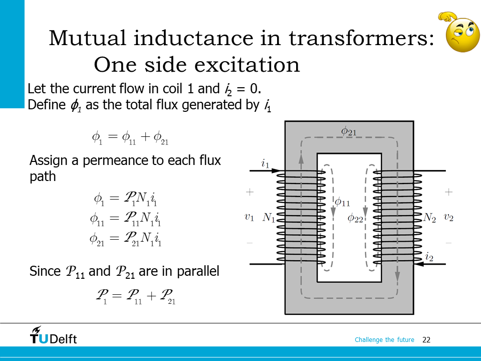
To study how to quantify the coupling between the two coils, let us do a thought experiment. Let current flow in coil 1 to be \(i_1\), and keep the second coil open, so \(i_2 = 0\). The total flux linked with coil 1 is composed of the flux links coil 2 through the magnetic core \(\phi_{21}\) and the part only links with coil 1 itself \(\phi_{11}\).
From the magnetic circuit principle we know
The permeance \(\mathcal{P}_{21}\) is corresponding to the main path of the flux, and \(\mathcal{P}_{11}\) is corresponding to the leakage path of coil 1.
Then the flux linkages of the two coils are
where \(\lambda_{21}\) represents the flux linkage linked by coil 2 caused by current in coil 1. The coil 2 itself does not generate flux since it is open at the moment. \(\mathcal{P}_{21}\) is the permeance of the magnetic circuit path from coil 1 to coil 2.
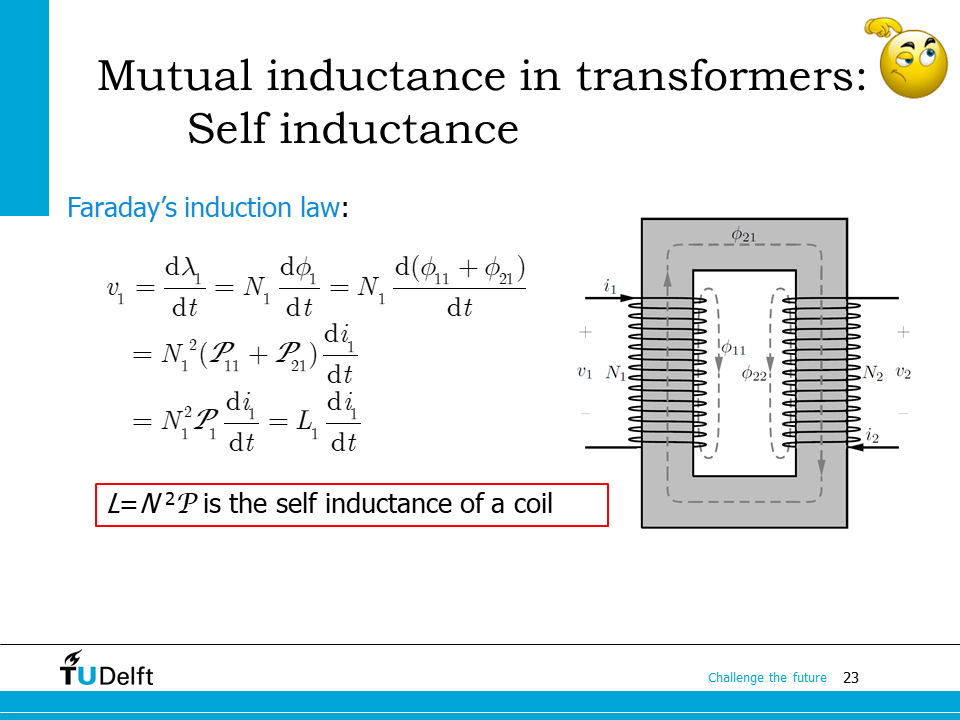
Then based on Faraday’s law, we are able to derive the voltage and the inductance of coil 1, which are
\(L_1\) is called self inductnace coil 1 since it corresponds to all flux linked with coil 1 itself.
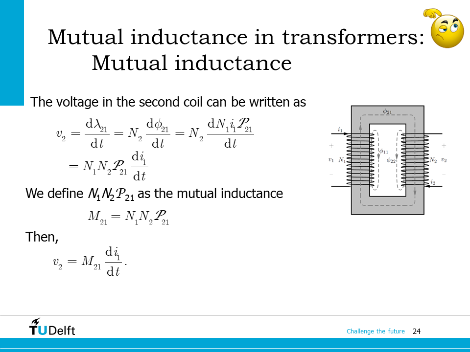
Similarly, according to Faraday’s law, there is also voltage induced in coil 2.
Here we define \(M_{21} = N_1N_2\mathcal{P}_{21}\) as the mutual inductance from coil 1 to coil 2, since it represents the capability of coil 1 induces voltage in coil 2.
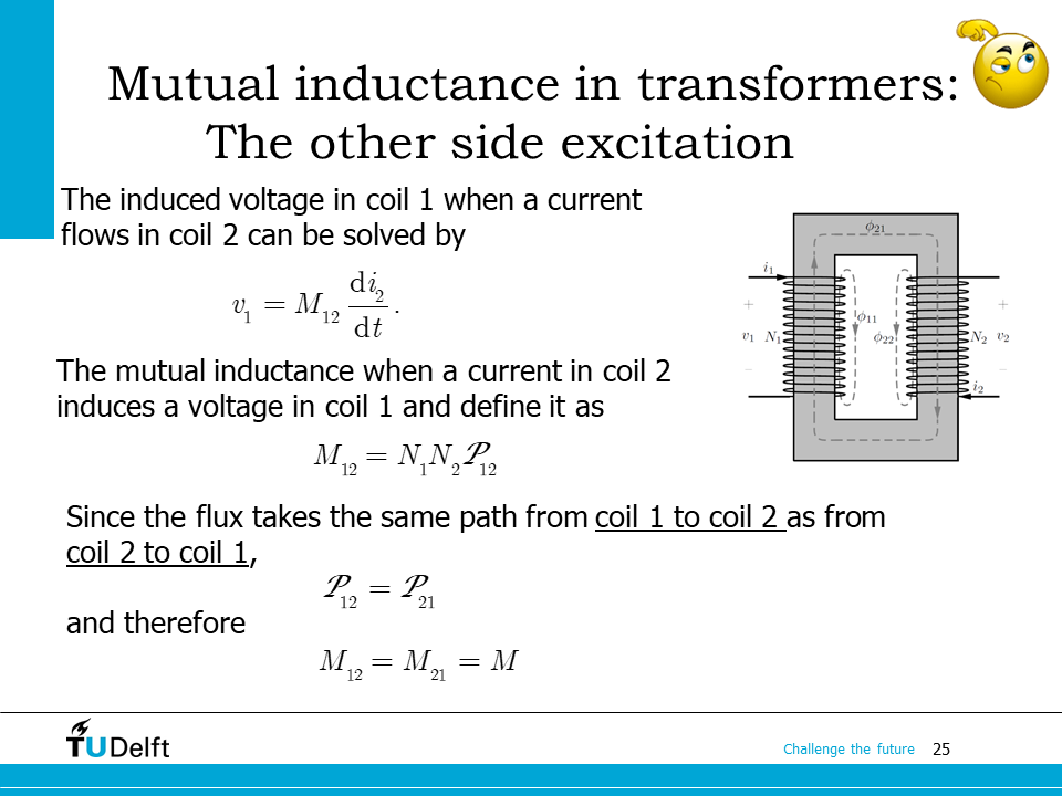
Similarly, by setting coil 1 open, and inject a current \(i_2\) in coil 2, following the current and voltage definitions given in the figure, the voltages in coil 1 and coil 2 can be solved as
Here we define \(M_{12} = N_1N_2\mathcal{P}_{12}\) as the mutual inductace from coil 2 to coil 1. \(L_2\) is the self inductance of coil 2.
Apparently the flux path from coil 1 to coil 2 are exactly the same as that from coil 2 to coil 1, so the two mutual inductance is the same
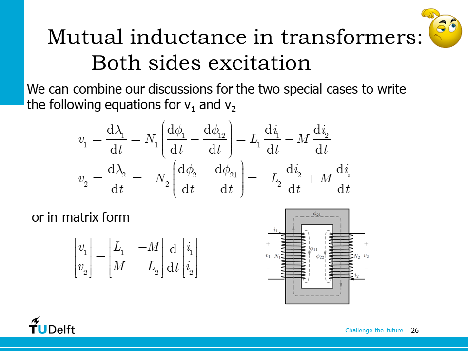
In the above two thought experiments, one of the coils is kept open. Now let’s check a more general case, where both \(i_1\) and \(i_2\) are non zero.
Following the notation given in the figure on the slide, the flux linkages of the two coils should include the contributions from coil itself and the other coil
Then the voltage equations can be written as
or as the matrix form shown on the slide.
Attention
There are many different definitions for the current and voltage directions and many textbooks will choose a different secondary voltage definition such that the signs in the second row of the matrix reverses. Here we choose to follow the definition shown on the slide so that is it consistent with the standard definitions of an ideal transformer.
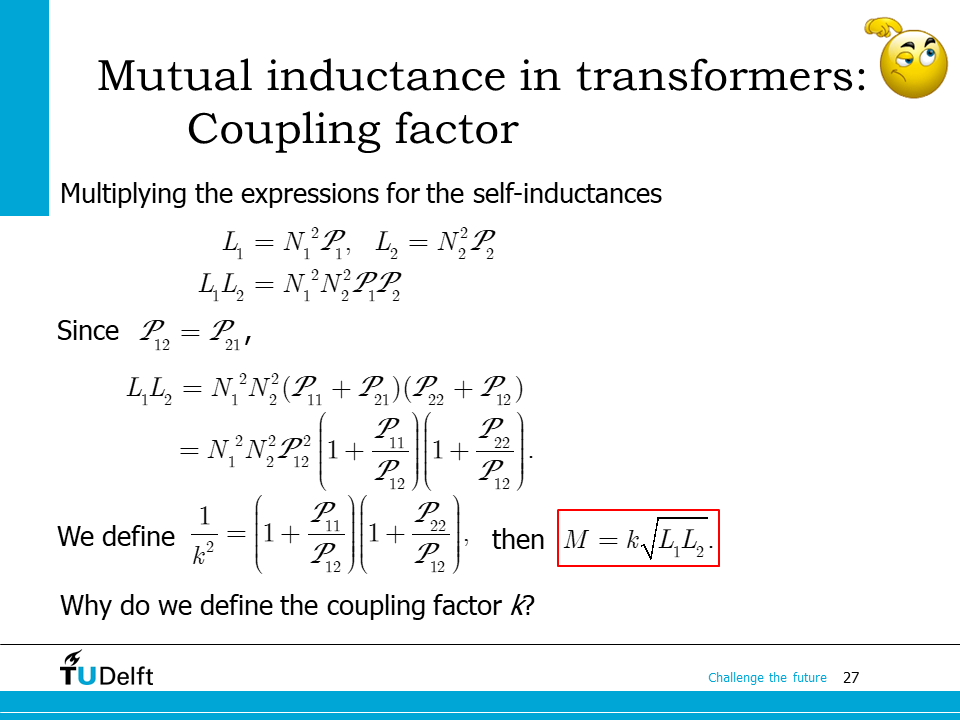
The two voltage equations or their matrix form do not give an intuitive feeling about how well the two coils are coupled. Hereby we introduce the concept of coupling factor.
The product of the two self inductances expressed by permeance is shown on the slide. Keeping in mind that the magnetic circuit remains the same, so \(\mathcal{P}_{12} = \mathcal{P}_{21}\). By taking \(\mathcal{P}_{12}\) out of the parentheses, we have
Here the coefficient of coupling, or coupling coefficient \(k\) is defined as \(1/\sqrt{(1+\mathcal{P}_{11}/\mathcal{P}_{12})(1+\mathcal{P}_{22}/\mathcal{P}_{12})}\). Therefore we have \(M = k\sqrt{L_1L_2}\).
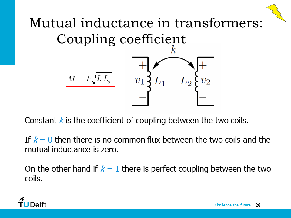
\(k = 0\) means there is no common flux between the two coils and the mutual inductance is zero. \(k = 1\) means the coupling between the two coils is perfect and the leakage flux \(\phi_{11} = \phi_{22} = 0\). The allowable range for the coefficient of coupling is \(0 \leq k \leq 1\). In practical systems it is impossible to obtain \(k=1\). However, in certain cases, such as power transformers, where the intention is to maximize the coupling, it is possible to achieve a coupling coefficient in excess of 0.99. In contactless power transfer applications, however, \(k\) can be as low as several percents.
Using the voltage equations and mutual inductance is not always straightforward for circuit analysis, since we have to deal with two equations. It is handy for analysis of coupled circuits if we introduce the leakage and magnetising inductances.
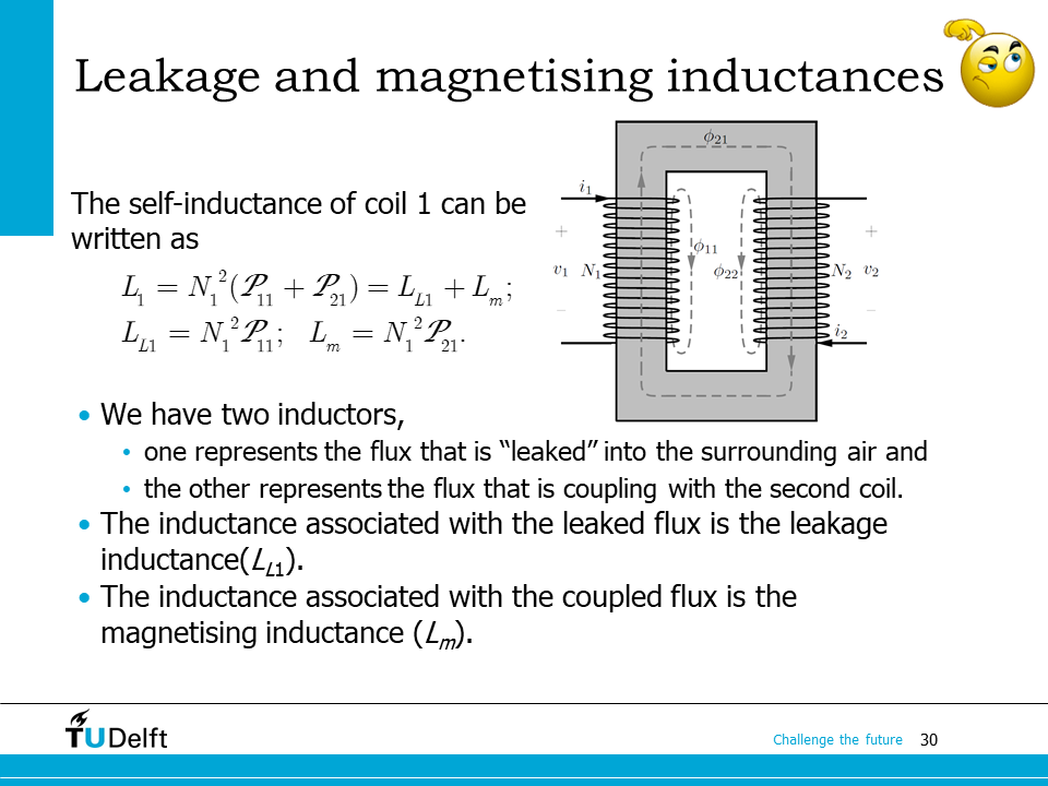
We know the self inductance of coil 1 can be written as the sum of two parts: the one corresponds to the flux which only links coil 1 itself \(N_1^2\mathcal{P}_{11}\), and the one corresponds to the flux couples with both coils \(N_2^2\mathcal{P}_{21}\).
THe former one represents the flux which is leaked to the surroundings, so it is defined as the leakage inductance \(L_{L1}\), and the second one is associated with the coupled flux which magnetise the magnetic core, so it is defined as the magnetising inductance \(L_m\).
This way we are able to divide the coil 1 inductance into two inductances: magnetising inductance and leakage inductance.
Similar approach can be applied to coil 2.
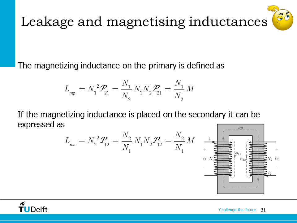
In practice, it is difficult to measure the permeance \(\mathcal{P}_{11}\) or \(\mathcal{P}_{21}\), so it is difficult to obtain the value of \(L_m\) and \(L_{L1}\) from permeances. However, recalling the definition of the mutual inductance and coupling coefficient, we are able to obtain the relative relationship between the inductances.
For the primary side (coil 1), the magnetising inductance is
Using the same approach, if magnetising inductance is placed on the secondary side, we have the secondary magnetising inductance as
You may notice that
which is corresponding to the impedance transfer ratio when the magnetising inductance is referred from the secondary side to the primary side.
Based on the defined magnetising inductance and the leakage inductances, we will introduce the equivalent circuit of the non ideal transformer.
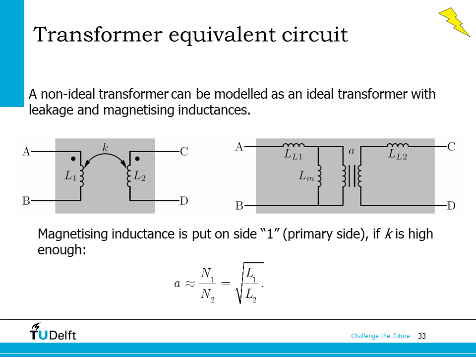
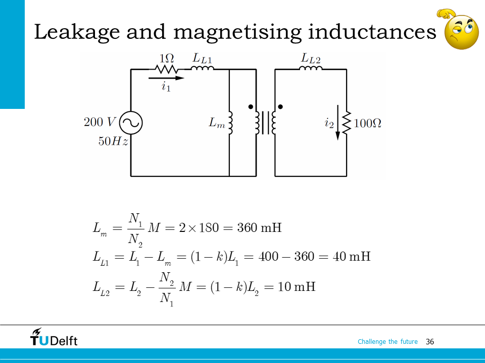
Now we can approximate a non ideal transformer by adding the magnetising inductance and the leakage inductances to an ideal transformer, as shown on the slide.
If we assume the coupling coefficient \(k\) is high enough, since \(L=N^2\mathcal{P}\), the transformer ratio of the ideal transformer can be approximated as the square root of the self inductance ratio
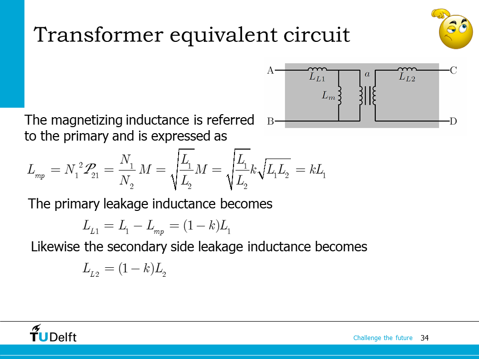
Then the magnetising inductance is calculated as
The primary leakage inductance is therefore
Likewise, the secondary side inductance is solve
16.3. Example#
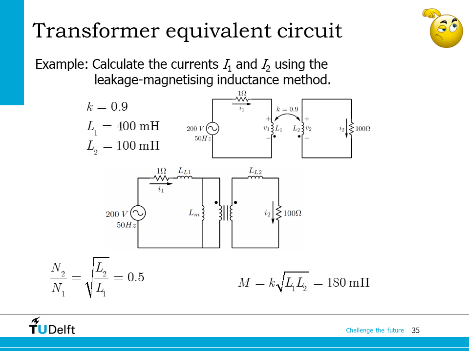
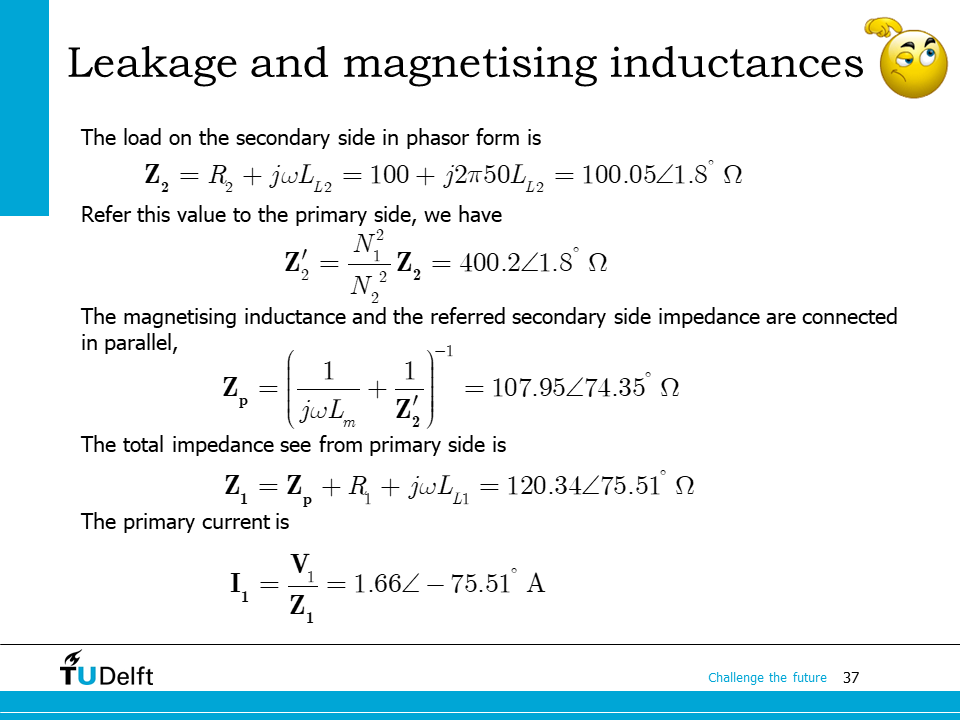
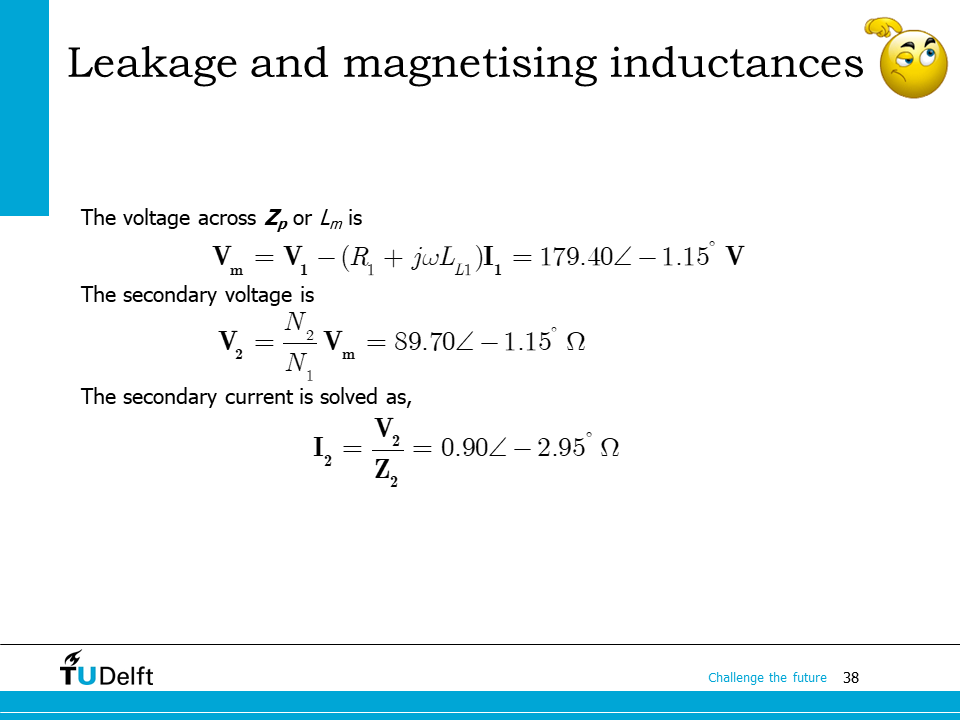
Then let us use this example to practice problem solving with equivalent circuit. Please try to work it out yourself and click the block below for the detailed answer. The Python code below also shows the calculation procedure.
Click here for solution
Show code cell source
%reset -f

import numpy as np
from sympy import *
import cmath
from IPython.display import display, Markdown, Math, Latex

k  = 0.9
L1 = 400.0e-3
L2 = 100.0e-3
Vp = 200.0
R1 = 1.0
R2 = 100.0
f  = 50.0
omega = 2*np.pi*f

M  = k*np.sqrt(L1*L2)

a  = sqrt(L1/L2)

# first use the coupled inductors method

i_1, i_2 = symbols('i_1, i_2')
eq1 = Vp-i_1*R1-1j*omega*(i_1*L1-i_2*M)
eq2 = 1j*omega*M*i_1 - 1j*omega*L2*i_2 - R2*i_2

sols = solve([eq1,eq2], [i_1,i_2])

I_1  = sols[i_1].evalf()
I_2  = sols[i_2].evalf()

print('From the coupled inductors method:')
display(Math('$\mathbf{{I_1}}={:.2f}\\angle{:.2f}^\circ$'.format(abs(I_1), cmath.phase(I_1)/np.pi*180)))
display(Math('$\mathbf{{I_2}}={:.2f}\\angle{:.2f}^\circ$'.format(abs(I_2), cmath.phase(I_2)/np.pi*180)))

# then use the equivalent circuit method

Lm  = k*L1
LL1 = (1-k)*L1
LL2 = (1-k)*L2

Z2  = 1j*omega*LL2+R2

# refer secondary impedance to primary side
Z2_prime = Z2*a**2

Zm  = 1j*omega*Lm
Z1  = R1 + 1j*omega*LL1

# total impedance
Ztot = Z1 + 1/(1/Zm+1/Z2_prime)
I1   = Vp/Ztot

# voltage across Lm
Vm   = (1/(1/Zm+1/Z2_prime))/Ztot*Vp
# referred to secondary side
V2   = Vm/a
I2  = V2/Z2

print('From the equivalent circuit method:')
display(Math('$\mathbf{{I_1}}={:.2f}\\angle{:.2f}^\circ$'.format(abs(I1), cmath.phase(I1)/np.pi*180)))
display(Math('$\mathbf{{I_2}}={:.2f}\\angle{:.2f}^\circ$'.format(abs(I2), cmath.phase(I2)/np.pi*180)))
From the coupled inductors method:
From the equivalent circuit method:
In the code above, we solved the problem using two approaches: 1) analyse it as coupled inductor and solve the voltage equations, 2) use the equivalent circuit to simplify the circuit.
Apparently both methods give use the same results. The equivalent circuit is easier for hand calculation since it does not require linear equation solving.
16.4. Transformer parameter measurements#

The circuit elements in the equivalent circuit are not directly accessible, however, it is possible to obtain their values indirectly by doing some tests.
First an open circuit test is carried out. We supply the primary side with rate voltage \(V_{1o}\), then measure the input current \(I_{1o}\) and secondary side open circuit voltage \(V_{2o}\). The open circuit reactance \( X_{1o}\) can be obtained from \(V_{1o}\) and \(I_{1o}\). From them the following equations are obtained
Then a short circuit test is carried out. We short circuit the secondary side, and supply primary side with a rated current \(I_{1s}\). Then primary side voltage \(V_{Is}\) is measured. The short circuit reactance \(X_{1s}\) can be obtained from \(V_{1s}\) and \(I_{1s}\). If we assume \(k\) is high enough, we can reasonably neglecting current going through \(L_m\), so we have
There are three equations but four unknows, we need to make further assumptions to make it solvable. One approach is to assume \(\mathcal{P}_{11} = \mathcal{P}_{22}\), i.e., the leakage paths have the same permeance on both sides, so we have
Then we are able to solve all four parameters in the equivalent circuits from measurement results.
The method described above is a simplified version based on the standard approach. In practice, the measurements are more complicated since we have to deal with more non-ideal factors including winding resistances and core losses etc.