17. Mechanical Energy Conversion

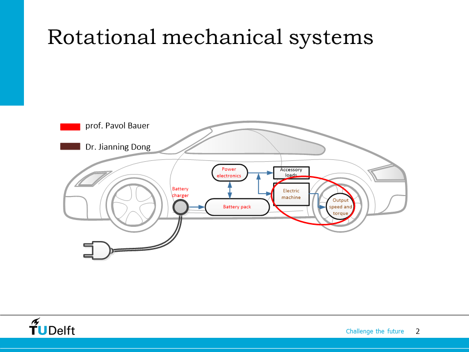
In this module, the mechanical energy conversion is studied. If we use the electric vehicle as an example, this module studies the transmission part of the vehicle, which is located between the electrical machine and the wheels.

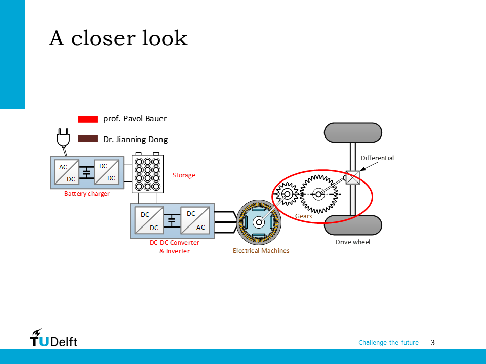
If we take a closer look, the mechanical energy conversion happens in the system consists of electrical machines, gears, differential and wheels.

In this lecture, we will make an analogy between the electrical energy conversion and the mechanical energy conversion, i.e., the inertia will function as a “mechanical inductance”, while the gearbox can be treated as a “mechanical transformer”.

We will also study the mathematical models of various mechanical components, and study their dynamic and steady state behaviour based on the models.

17.1. Electrical drives

Before coming to the mechanical system, the electrical drive should be studied. It is essential because in modern energy conversion systems, we rarely use mechanical energy directly since it is difficult to regulate. Instead, we convert the mechanical energy from prime movers (e.g., diesel engine) first to electrical energy using generators, then use electrical drive to drive the mechanical load. This configuration improves the overall efficiency and provides flexibility.

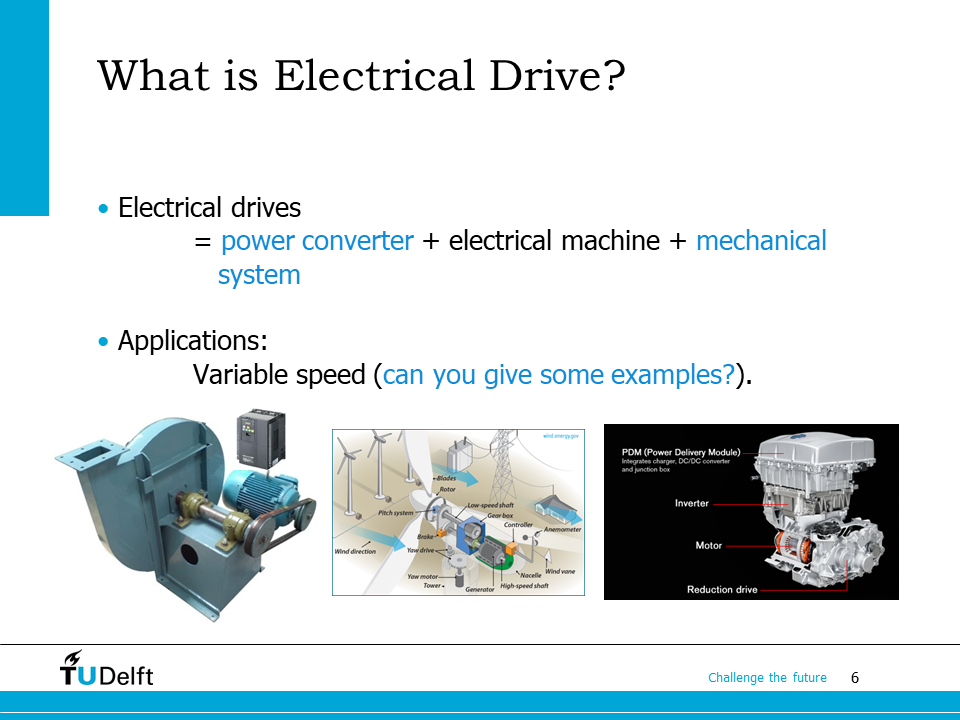
The core of an electrical drive is the electrical machine. To control the speed and torque of the electrical machine, a power converter is used to regulate the voltage and frequency feeding the machine. To match the characteristic of the electrical machine to the load, a mechanical system, e.g., a gearbox, can be used.

The electrical drive is extensively used in applications which require variable speed. There are some examples including the electric vehicles, wind turbines, etc.

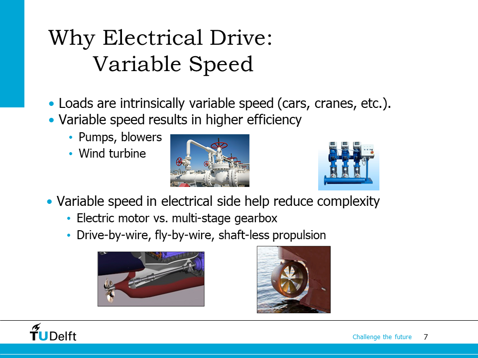
Variable speed electrical drive is needed because of several reasons:

• Some loads are intrinsically variable speed, for example, electric cars, cranes, etc.

• Some system performs more efficiently if variable speed is used. For example, a wind turbine needs to change the rotating speed according to the wind speed to achieve the optimal tip speed ratio (TSR); a pump can control the flow rate by changing the speed more efficiency compared to that using a valve.

• By using a variable speed drive, the power transmission system can be simplified. For example, the diesel engine only achieves optimal efficiency in very narrow speed range, to match the load, a multi-stage gearbox is needed. However, if an electrical drive is used, diesel engine can operate at the optimal speed to generate electricity via a generator, then the electricity is used by the variable speed drive to turn the load, so that the gearbox can be omitted. It is even possible to transmit the power without using a big shaft, if the electric motor is coupled to the propeller directly — the power can be more flexibly transmitted by electric cables.

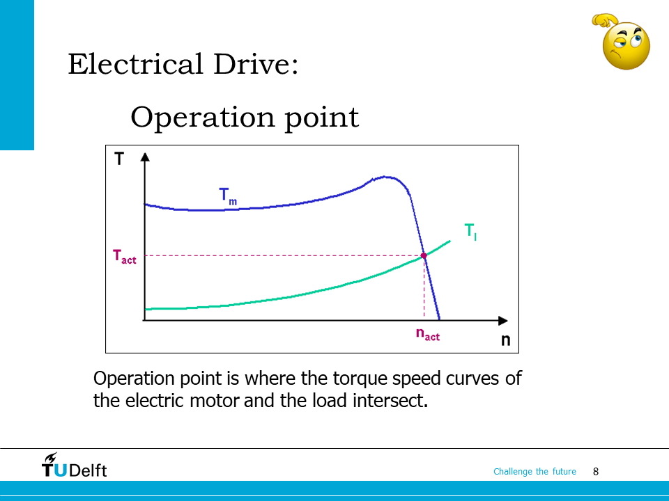
The torque-speed characteristic is an important concept for both the electrical drive and the load. If both torque-speed characteristics are plotted in one graph, the intersection point of them will be the operation point. By placing the mechanical system between the load and the electrical drive, the torque-speed characteristic of the load can be changed, so that it fits better with the electrical drive. The mechanical system in between in this case works like a transformer in the electrical circuit.

17.2. Linear and rotational dynamics

First we study the linear mechanical system and the rotational system, and how to convert between the linear motion and the rotational motion.

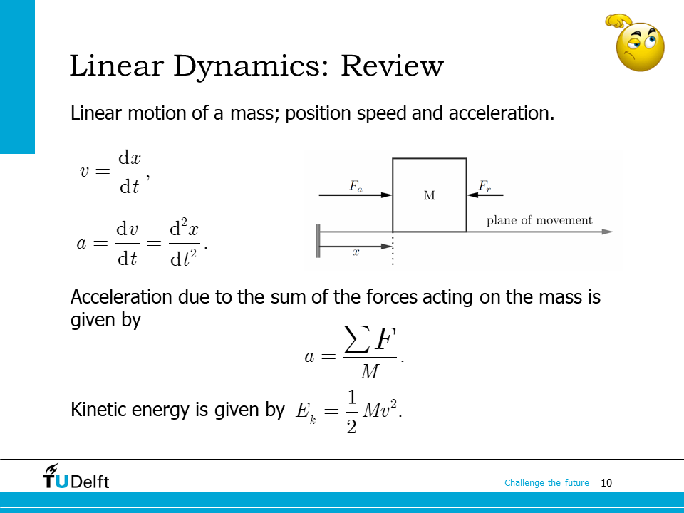
For the linear motion, if the displacement is defined as \(x\). The speed \(v\) and the acceleration \(a\) will be

\[ v = \frac{\mathrm{d} x}{\mathrm{d} t};\quad a = \frac{\mathrm{d} ^2x}{\mathrm{d} t^2}. \]

Then we are able to obtain the differential equation to describe the dynamics of the linear mechanical system by applying Newton’s Law.

\[ a = \frac{\mathrm{d} v}{\mathrm{d} t} = \frac{\Sigma F}{M}. \]

where \(\Sigma F\) is the total force applied on the mass \(M\).

The kinetic energy stored in the moving mass is then calculated as

\[ E_k = \frac{1}{2}Mv^2. \]

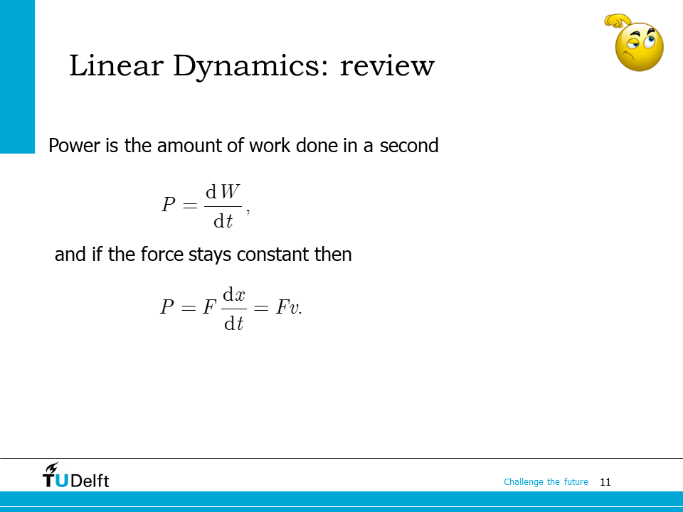
From the store kinetic energy \(E_k\), or the amount of work done by the force \(W\), we could also derive the power applied by the force to the mass

\[ P = \frac{\mathrm{d} E_k}{\mathrm{d} t} = \frac{\mathrm{d} \frac{1}{2}Mv^2}{\mathrm{d} t} = Mv\frac{\mathrm{d} v}{\mathrm{d} t}. \]

If the force stays constant, i.e., \(F = M\frac{\mathrm{d} v}{\mathrm{d} t}\) is a constant, the power equation becomes

\[ P = Fv. \]

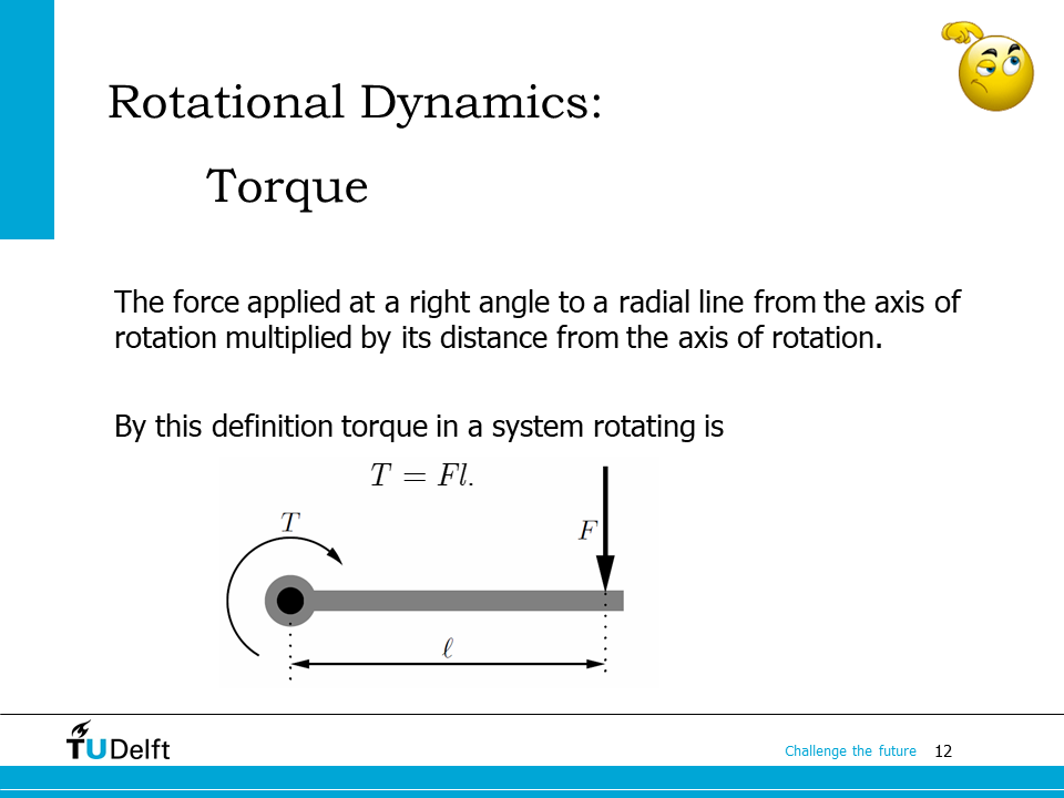
Then let us move on to the analysis of the rotational system. By applying a force \(F\) at a right angle to a radial line for the axis of rotation, the torque is defined as

\[ T = Fl. \]

where \(l\) is the length of the torque arm, and the direction of \(l\) should be perpendicular to the direction of the force.

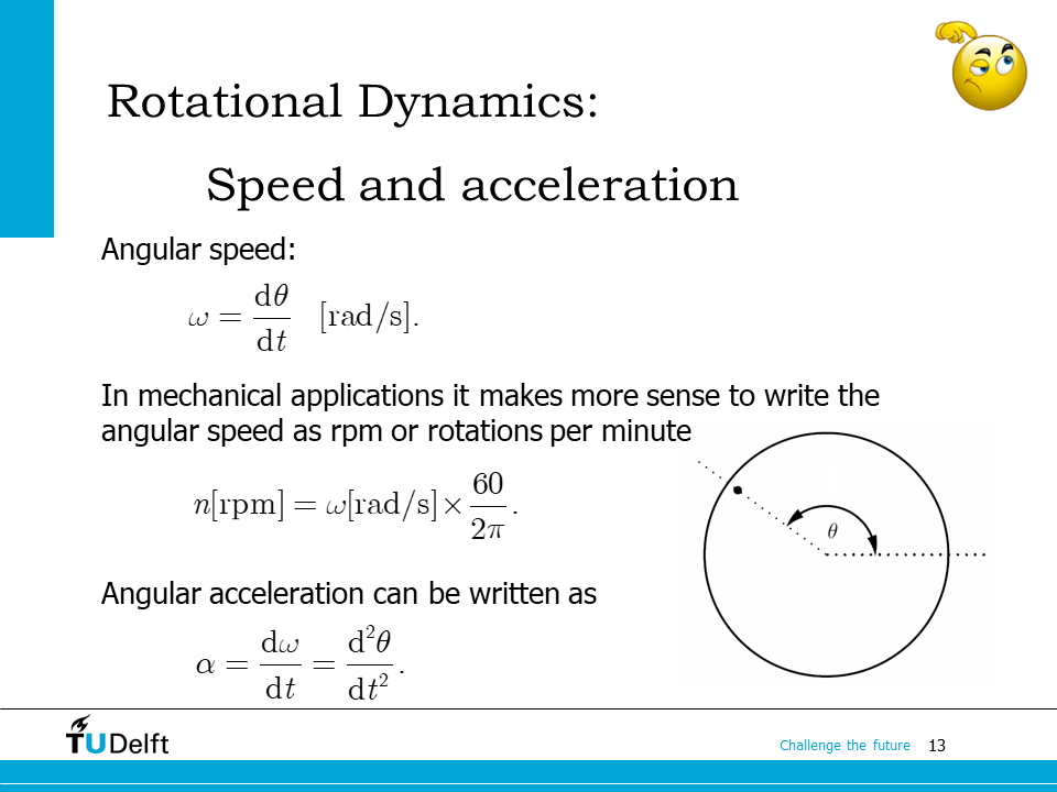
Similar to its linear counterpart, the “rotational displacement” should be represented by the rotational angle \(\theta\). The speed becomes the angular speed \(\omega = \frac{\mathrm{d}\theta}{\mathrm{d} t}\), in the unit of [rad/s]. When we are dealing with machines, the unit of revolutions per minute (rpm) or [r/min], is more often used. To convert the two from each other, we consider there are \(2\pi\) radians per revolution, and 60 seconds per minutes, so

\[ \omega = \frac{2n\pi}{60}. \]

The angular acceleration \(\alpha\) can also be defined

\[ \alpha = \frac{\mathrm{d} \omega}{\mathrm{d} t} = \frac{\mathrm{d}^2 \theta}{\mathrm{d} t^2}. \]

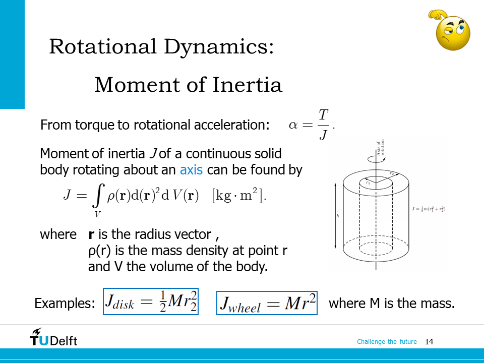
For the rotational motion, the different equation can also be derived from Newton’s Second Law,

\[ \alpha = \frac{\mathrm{d} \omega}{\mathrm{d} t} = \frac{T}{J}. \]

where \(J\) is the moment of inertia. The moment of inertia \(J\) of a solid body is calculated from the mass density of it \(\rho\) and its shape by

\[ J = \int_V\rho(\mathbf{r})\mathrm{d}V(\mathbf{r}) \quad [\mathrm{kg\cdot m^2}] . \]

where \(\mathbf{r}\) is the radius vector and \(V\) is the volume of the body.

If the body is rotating around the \(z\)-direction perpendicular to the cross sectional plane, for a disk with uniformly distributed mass, its moment of inertia is

\[ J_{disk} = \frac{1}{2}Mr_2^2, \]

and for a wheel is

\[ J_{disk} = Mr_2^2. \]

where \(M\) is the total mass, \(r_2\) is the external radius, \(r\) is the radius of the wheel.

For the thick-walled cylindrical tube with open ends shown in the slide, with inner radius \(r_1\) and outer radius \(r_2\),

\[ J = \frac{1}{2}M(r_1^2+r_2^2). \]

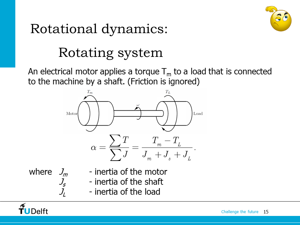
The dynamics of several bodies coupled to the same shaft can be described in the same way by summing up the torques and moments of inertia on the shaft.

As shown on the slide, there is a motor delivering torque \(T_m\) with the moment of inertia \(J_m\). The load connected to shaft has a load torque of \(T_L\) and a moment of inertia of \(J_L\). The moment of inertia of the shaft is \(J_s\). Therefore, the angular acceleration of the common shaft system is

\[ \frac{\mathrm{d} \omega}{\mathrm{d} t} = \frac{\Sigma T}{\Sigma J} = \frac{T_m-T_L}{J_m+J_s+J_L}. \]

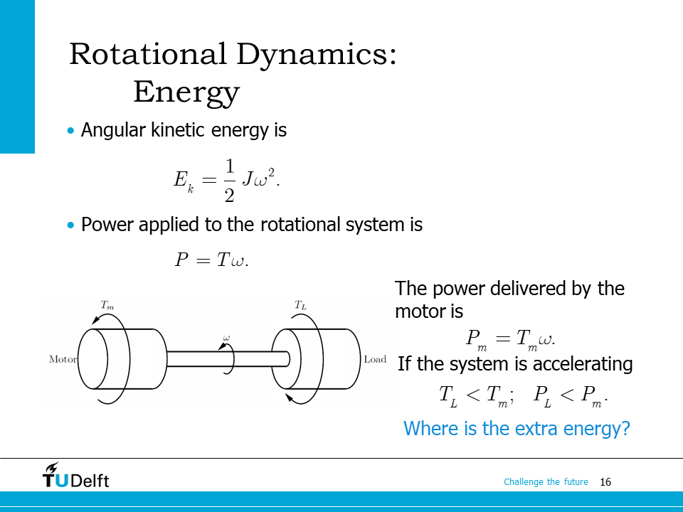
Similar to the linear system, the angular kinetic energy is

\[ E_k = \frac{1}{2}J\omega^2. \]

The power applied to the rotational system is the derivative of the stored energy, which is

\[ P = T\omega. \]

As shown in the example on the slide, the power delivered by the motor is \(P_m = T_m \omega\). If the system is accelerating, \(T_L < T_m\) holds. The power to accelerate the system is

\[ P_m-P_L = (T_m-T_L)\omega, \]

which will be accumulated in the kinetic energy of the rotational system.

So far we reviewed the linear and rotational dynamics. Now let us study how various rational systems or linear systems couple with each other.

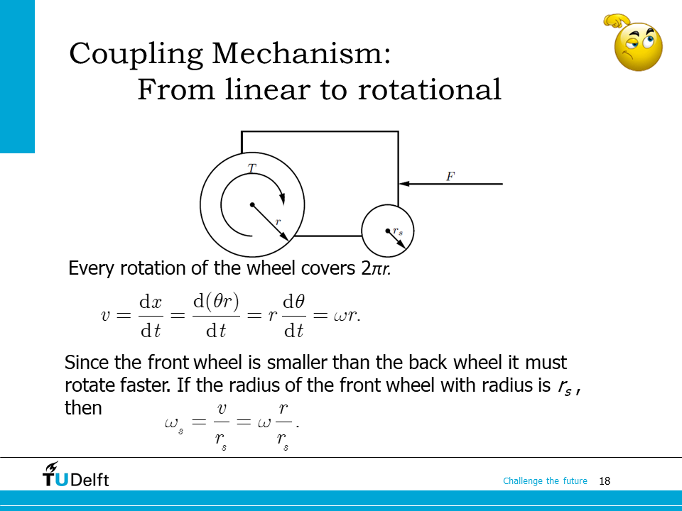
This topic can be elaborated with the vehicle shown on the slide. It has two wheels with different radii \(r\) and \(r_s\). When the vehicle is moving at a speed \(v\) in the horizontal direction. The linear speed on the surface of the two wheels is also \(v\). If we define the linear displacement of the vehicle as \(x\), then we have

\[ v = \frac{\mathrm{d} x}{\mathrm{d} t}. \]

\(x\) can be related to the angle the two wheels rotate \(\theta\) and \(\theta_s\), so

\[ x = \theta r = \theta_s r_s. \]

Then we have

\[ v = \frac{\mathrm{d} x}{\mathrm{d} t} = \frac{\mathrm{d} \theta r}{\mathrm{d} t} = \frac{\mathrm{d} \theta_s r_s}{\mathrm{d} t}. \]

Since \(\omega = \mathrm{d}\theta/\mathrm{d} t\), we have

\[\begin{split} \begin{align} \omega_s r_s &= \omega r, \quad\text{or} \\ \frac{\omega_s}{\omega} &= \frac{r}{r_s}. \end{align} \end{split}\]

which means the smaller wheel should rotate faster than the larger wheel. The two wheels couple to each other in a way similar to currents in an ideal transformer.

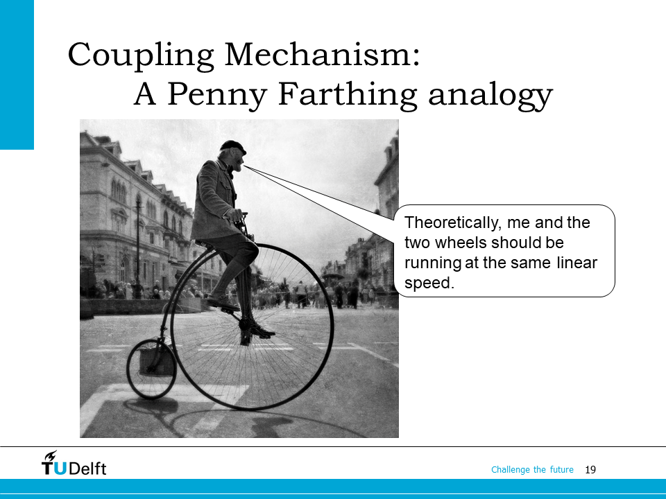
This coupling principle is applied in many applications. Here it shows an early ancestor of the bike we ride everyday, which is called penny farthing or high wheeler. It was popular in 1870s and 1880s. At that time, we do not have mature chain transmission technology, so the front wheel is directly driven by our leges. We have to use a large front wheel to provide high speed (for the same angular speed provided by the rider, the larger the wheel, the faster). The larger wheel also provides good shock absorption.

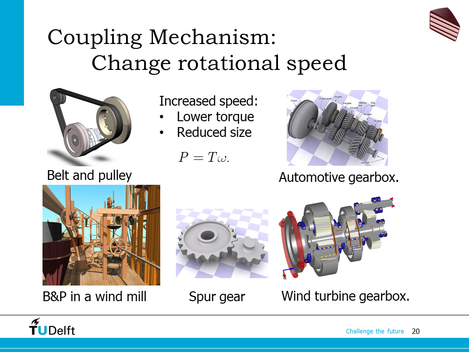
Thanks to modern mechanical transmission systems, we are able to transform speed more flexibly, as shown on the slide. So in modern bikes, we rely on gears and chains, or pulleys and belt for transmission. The two wheels can have the same size thanks to them.

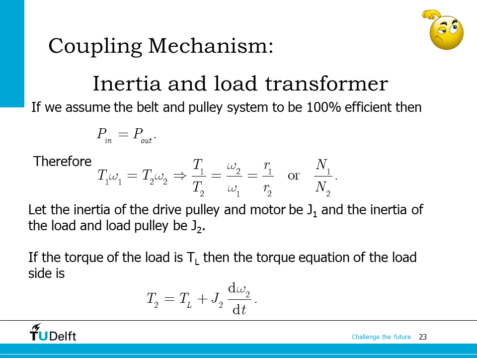
For various coupling mechanisms shown here, we should bear in mind that, because of the first law of thermodynamics, the coupling mechanisms here do not create new energy. So the power should be equivalent on both sides. In practice, part of the mechanical energy will be converted to heat because of friction, so the transmission efficiency is always below one.

If we neglect the loss, on the primary and secondary sides of the transmission, we have

\[ P_1 = P_2 = T_1\omega_1 = T_2\omega_2, \]

so the torque transfer ratio is the inverse of the angular speed transfer ratio.

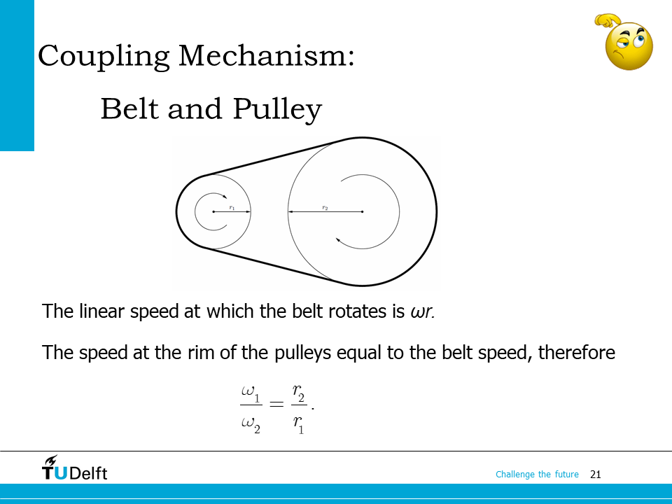
Here it shows a simple pulley and belt system. For the two belts with radii \(r_1\) and \(r-2\), when they are coupled to the same pulley, the linear speed on their surfaces should be the same, so we have

\[ \frac{\omega_1}{\omega_2} = \frac{r_2}{r_1}. \]

In ideal case, when the loss is neglected, the torque transfer ratio would be

\[ \frac{T_1}{T_2} = \frac{r_1}{r_2}. \]

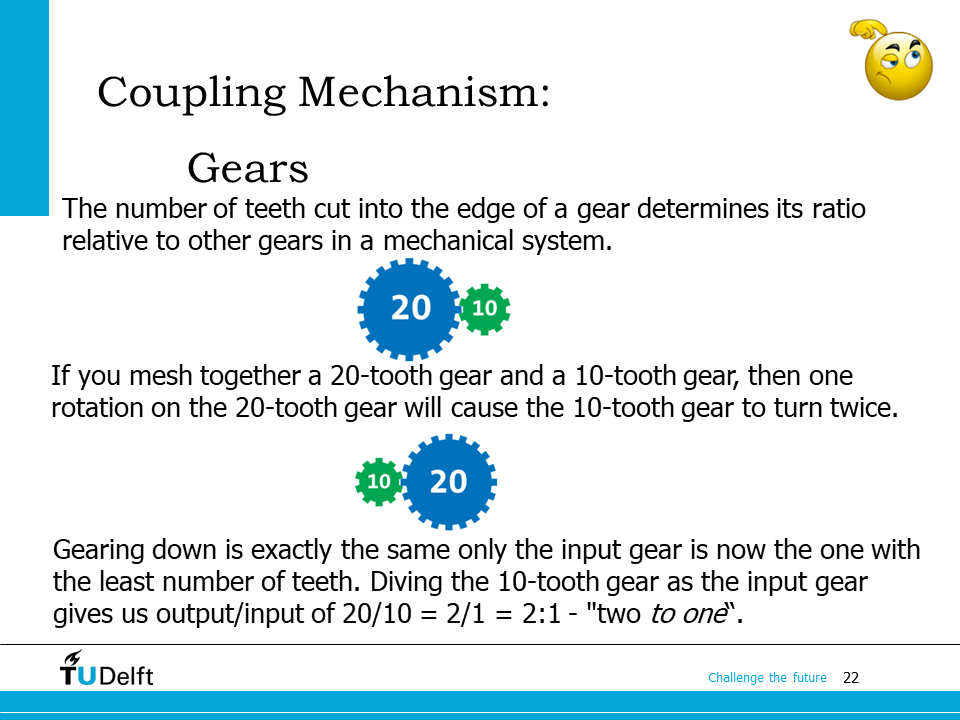
Similarly, we are able to derive the angular speed and torque transfer ratios. When two gears are coupled together with number of teeth \(N_1\) and \(N_2\) respectively, they have to turn the same number of teeth during a specific period, so the angular speed ratio becomes

\[ \frac{\omega_1}{\omega_2} = \frac{N_2}{N_1}. \]

Hence the gear with larger number of teeth rotates slower than the one with less number of teeth. The torque transfer ratio is the inverse of it

\[ \frac{T_1}{T_2} = \frac{N_1}{N_2}. \]

Here it summarises the two coupling mechanisms under the ideal conditions (100% efficiency).

Now let’s assume that there is a motor installed directly on the shaft of drive pulley 1, and the load is installed on the shaft of the load pulley 2. Their moments of inertia are \(J_1\) and \(J_2\) respectively.

Then for the load pulley 2 and the Newton’s Second Law of Motion, we have the following differential equation to describe its dynamics

\[ T_2 -T_L = J_2\frac{\mathrm{d}\omega_2}{\mathrm{d}t}, \]

where \(T_2\) is the driving torque transferred to the load pulley 2.

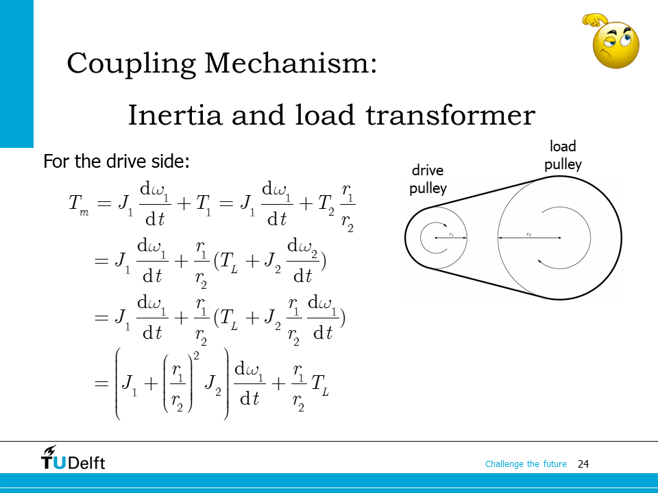
If the system is viewed from the drive pulley 1, and \(T_m\) is the torque applied on pulley one from the motor, the differential equation to describe the dynamics of the primary pulley is

\[ \newcommand{\diff}{\mathrm{d}} T_m = J_1\frac{\diff \omega_1}{\diff t} + T_1, \]

where \(T_1\) is the load torque applied to the primary pulley.

We know \(T_1/T_2 = r_1/r_2\), so the above equation becomes

\[ \newcommand{\diff}{\mathrm{d}} T_m = J_1\frac{\diff \omega_1}{\diff t} + T_2\frac{r_1}{r_2}. \]

Substituting the dynamic equation from the load pulley \(T_2 -T_L = J_2\frac{\mathrm{d}\omega_2}{\mathrm{d}t}\), we get

\[\begin{split} \begin{align} \newcommand{\diff}{\mathrm{d}} T_m &= J_1\frac{\diff \omega_1}{\diff t} + \left( T_L + J_2\frac{\diff\omega_2}{\diff t} \right)\frac{r_1}{r_2} \\ &= J_1\frac{\diff \omega_1}{\diff t} + \left( T_L + J_2\frac{r_1}{r_2}\frac{\diff\omega_1}{\diff t} \right)\frac{r_1}{r_2} \\ &= \left( J_1 + \left( \frac{r_1}{r_2} \right)^2 J_2 \right)\frac{\diff \omega_1}{\diff t}+\frac{r_1}{r_2}T_L. \end{align} \end{split}\]

As we can see from the derivations above, after placing the pulley and belt system in between the drive and the load, the load moment of inertia and torque seen from the drive side are both transferred, and the transfer ratios for the moment of inertia and the torque are \((r_1/r_2)^2\) and \(r_1/r_2\) respectively.

In practice, there is always energy loss in mechanical transmission, so the power on the load side would be lower than that from the drive side.

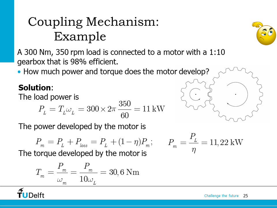
Now let us practice with the example here. A 1:10 gearbox between the motor and the load means the motor will rotate faster than the load because the number of teeth is less. Naturally, the torque on the motor side would be smaller.

The detailed calculation is shown on the slide. You may also refer to the Python script below.

From this example, we can see that by placing a gearing down gearbox between the motor and the load, the torque required by the motor will be reduced for the same load. Usually the volume and weight of an electric motor is proportional to its torque. That’s why in practice, we often use gearing down gearbox to drive the slow load with a higher speed motor to make the system more compact, e.g., in Tesla model S, a 1-speed fixed gear ratio (9.734:1 or 9.325:1) from the wheel to the motor is used.

Show code cell source Hide code cell source

import numpy as np
T_L = 300 # torque of load
n_L = 350 # r/min rotation speed of load
gear_ratio = 1.0/10.0 # gear ratio
eta = 0.98 # efficiency of the gearbox

omega_L = n_L/60.0*2*np.pi # convert from r/min to rad/s
P_L     = T_L*omega_L      # power on the load side
P_m     = P_L/eta          # power on the motor side

omega_m = omega_L/gear_ratio     # omega_L/omega_m = gear_ratio
T_m     = P_m/omega_m

print(f'The torque developed by the motor is {T_m:.2f} Nm.')

The torque developed by the motor is 30.61 Nm.

17.3. Analogy between electrical and mechanical principles

From above analysis, we can already see the mechanical coupling mechanisms work like transformers in an electrical system. Now let us summarise the analogy between them.

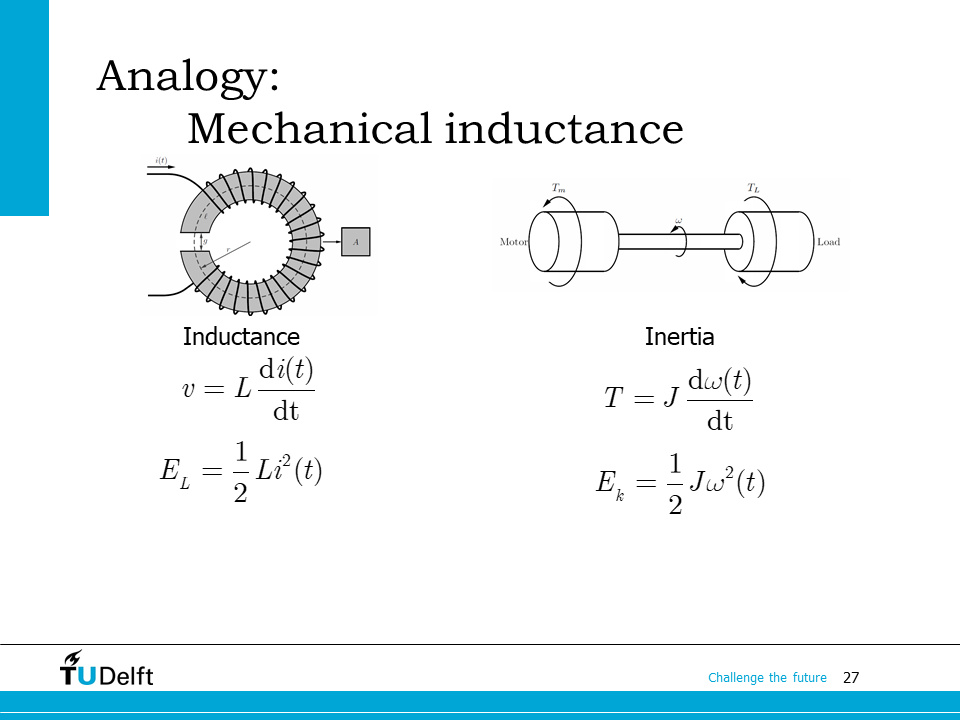
If we make an analogy from the voltage to the torque, then current in an electrical system becomes angular speed in the mechanical system. The inertia would function as a “mechanical inductance”, as shown on the slide.

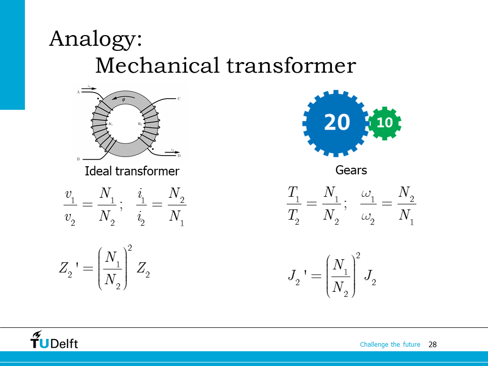
An ideal transformer functions as an impedance converter with a transfer ratio of the square of the turns ratio.

Similarly, a gearbox or a pulley and belt system function as a mechanical transformer, and it is able to convert the moment of inertia from the load side to the drive side, with a ratio of \((N_1/N_2)^2\) for a gearbox, or \((r_1/r_2)^2\) for a pulley and belt system.