18. Simple Electrical Machines#
From this lecture on, we will synthesise the knowledge on mechanical systems and electrical energy conversion to study the electrical machines.
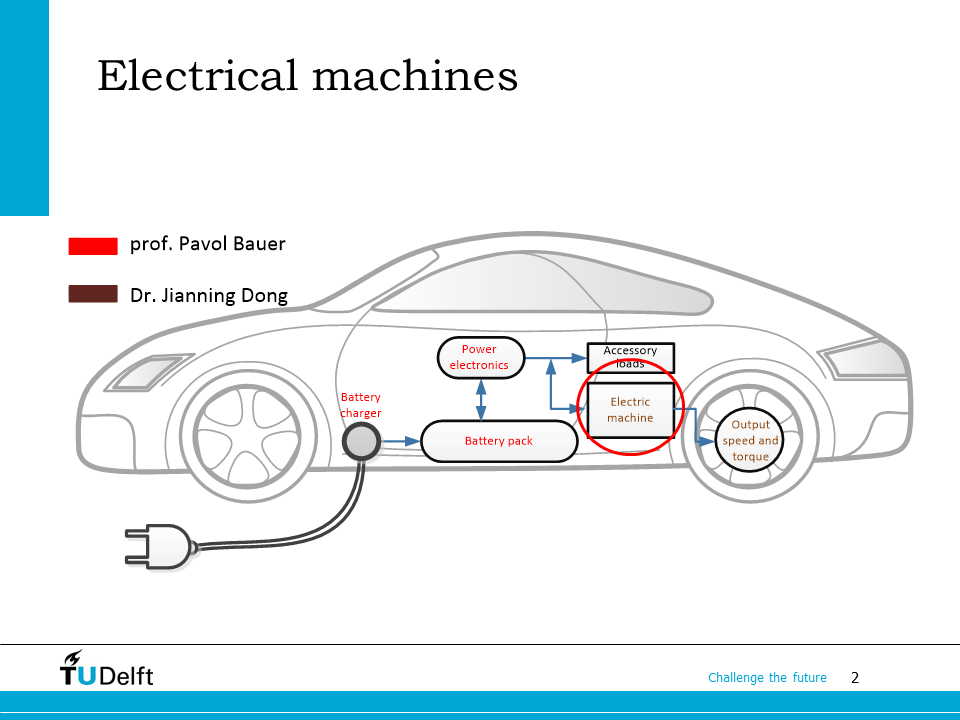
If we use the example of the electric vehicle again, the electric machine (or electrical machine) is placed between the power electronics converter and the wheels, to convert electrical energy stored in batteries to the mechanical energy to drive the vehicle.
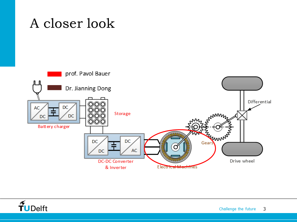
Here it shows the position of the electric machine in the overview of the electric powertrain.
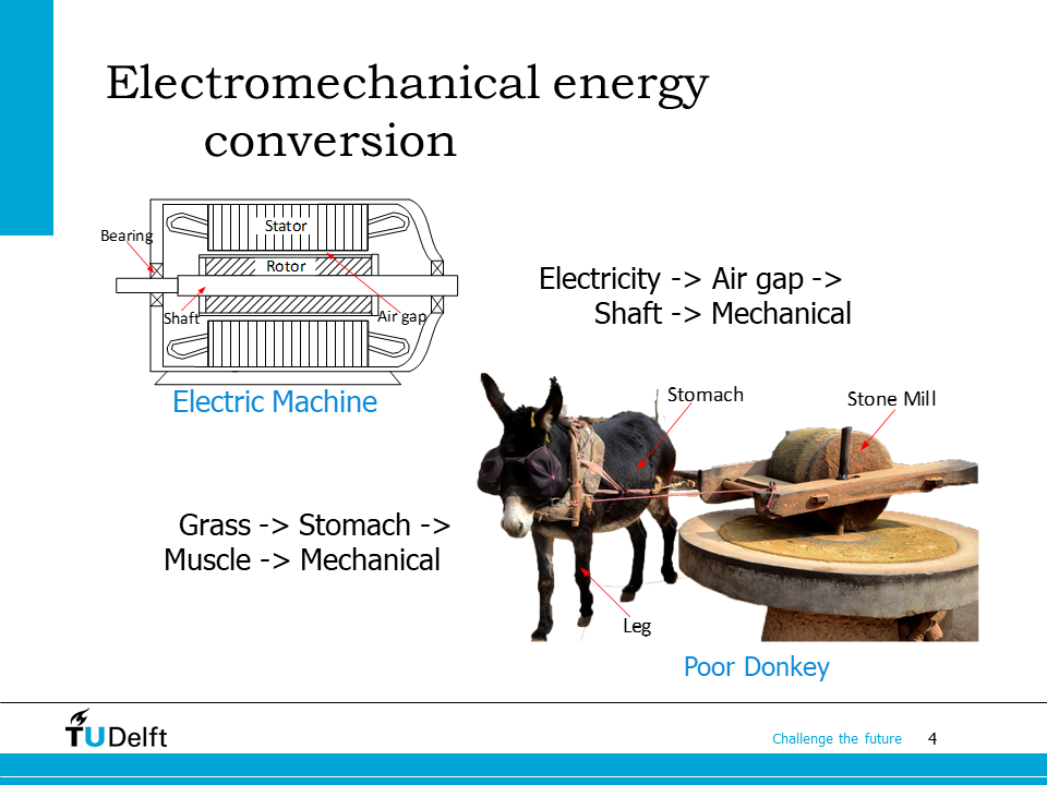
It is always nice to make analogies in learning. For a long time in history, animal engines have been extensively used to provide mechanical energy for repetitive rotational motion. As shown on the bottom right of the slide, a donkey mill is used for grinding grains. The donkey eats grass (biological energy), digests it in the stomach, and stores the energy inside its body. Then later on, the muscle of the donkey is used to deliver mechanical energy to push the stone mill. In this example, the donkey serves as a “bio-mechanical” machine.
The Dutch were smart enough to use “wind engine” to mill grains and pump water. But nowadays, they have been replaced with electric machines.
An electric machine is a device to convert energy between electricity and mechanical power, and in essence an electromechanical energy converter.
The structure of a rotating electric machine is shown on top left of the slide. It has a rotating rotor and a stationary stator. There is an air gap between the two. A shaft is mounted on the rotor to provide a mechanical interface to deliver or receive torque.
Unlike the animal engines, the electric machine is usually a bidirectional device, i.e., energy can be converted from electricity to mechanical output (motor) or vice versa (generator).
The transformer is often considered to be an electric machine, although they only convert electrical energy from one form to another and there is no moving part.
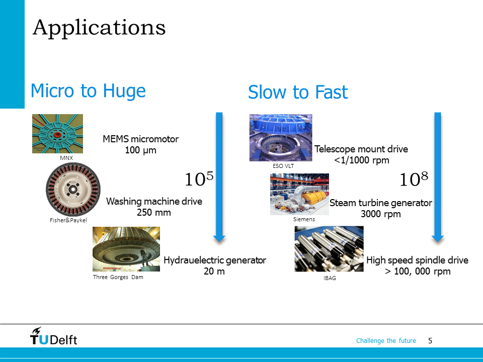
Electric machines have very extensive applications. Their sizes vary from hundreds of micrometers to tens of meters, and the rotation speeds vary from one thousands r/min to hundreds of thousand r/min.
Electric machines have become an indispensable part of our life. For example, there are several electric machines in our classroom: the cooling fan of the projector, the cooling fan of the PC, the ventilation system, and the drive system for the camera are all powered by electric machines. In our cellphones, there are also electric machines to produce vibrations.
This lecture is the first one in the electric machine part. After finishing it, we should be able to understand the electromechanical energy conversion process to enable the operation of the electric machine and carry out basic relevant calculations.
We will also study how to use constant magnetic field to produce a simple linear or a rotational machine. Afterwards, we will derive an equivalent circuit to model the simple electric machines.
We will start with the the simple case where a conductor is moving in a magnetic field.
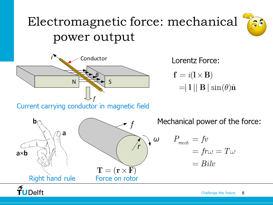
When a conductor carrying current \(i\) with length \(l\) is placed in a magnetic filed \(\mathbf{B}\), it would experience a force given by the Lorentz force law:
where \(\mathbf{l}\) is the length vector of the conductor, the direction of which indicates the current flow direction, \(\hat{\mathbf{n}}\) is unit vector perpendicular to the plane spanned by \(\mathbf{l}\) and \(\mathbf{B}\), \(\theta\) is the angle between the length vector \(\mathbf{l}\) and the flux density vector \(\mathbf{B}\).
Note
Cross product and dot product of vectors The equation are expressed in vectors. If \(\mathbf{a}\) and \(\mathbf{b}\) are both vectors, \(\mathbf{a}\times \mathbf{b}\) is used to denote the vector cross product, while \(\mathbf{a}\cdot \mathbf{b}\) indicates the vector dot product, a.k.a. dot product. When a cross product is applied, the result vector will have a direction governed by the right hand rule, as shown on the bottom left of the slide.
When the conductor is perpendicular to the magnetic field, the above vector calculation can be simplified into the scalar equation below
where \(B\), \(i\), \(l\) are the magnitude of the vectors above.
The direction of the force is then governed by the right hand rule:
Right hand rule for Lorentz force.
If the index finger is pointing in the direction of current flow, the middle finger in the direction of flux, then the thumb of the right-hand will point in the direction of the force.
If the conductor moves in the same direction of the force at the speed \(v\), we can obtain the power delivered by the force is
If we apply the force in tangential to the surface of a cylinder, through vector product as shown on the screen, we know the torque produced by the force is
If the cylindrical rotates at the angular speed of \(\omega\), we are able to obtain the power as
In the last slide, we know there is force produced when a current carrying conductor is exposed in a magnetic field, and if the conductor moves, there conductor will deliver mechanical power.
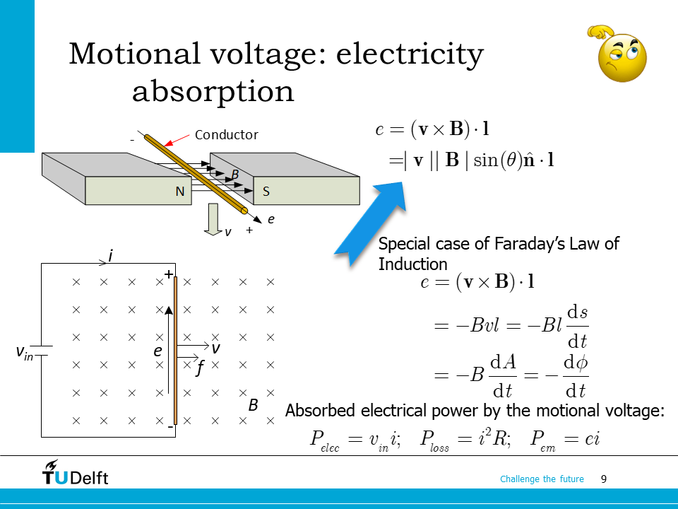
Here let us study the electrical behaviour of this conductor. When a conductor moves in the magnetic field, there will be voltage induced across the conductor, which can be solved as
where \(\mathbf{v}\) is the velocity of the conductor. The length vector \(\mathbf{l}\) is aligned with the direction of the wire, and the positive direction is defined as when the vector end points coincides with the wire end point. This voltage induced is called motional voltage or speed voltage. The equation above is in essence a special case of the Faraday’s Law of induction.
As we can see from the bottom left figure, When the three vectors \(\mathbf{v}\), \(\mathbf{B}\) and \(\mathbf{l}\) are perpendicular to each other, we will get
where \(\lambda\) is the flux linkage linked by the loop formed by the conductor, which is the same as the flux \(\phi= BA\) since there is only one turn, \(s\) is the distance the conductor moves.
The direction of the induced voltage can also be determined from the right hand rule:
Right hand rule for induced voltage
If the index finger is pointing in the direction of movement, the middle finger in the direction of flux, then the thumb of the right-hand will point in the direction of the positive terminal.
If we inject a current flow \(i\) into the induced voltage through an external source, there will be power absorbed by the induced voltage calculated by
which is called the electromagnetic power since it represent the power absorbed by the magnetic field induced voltage. The input power from the source is then
In most cases, there is resistance \(R\) in the circuit, so \(P_{elec}\neq P_{em}\), the loss is calculated as
Based on the two basic laws, let us construct the first simple electrical machine: a linear machine.
From above analysis, we know, if a current carrying conductor is moving in a magnetic field, and the direction vector of the conductor, the magnetic flux density vector, and the velocity vector of the conductor are perpendicular to each other, as shown in the bottom left figure, according to the Faraday’s Law of induction, the electrical power consumed by the conductor is
According to Lorentz force law, the mechanical power delivered by the force is
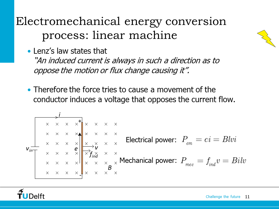
If we check both cases using the right hand rule, we will see that the induced voltage is opposing the input current, while the force is in the direction of the velocity, which means the force tries to cause a movement which induces a voltage that opposes the current flow. This is in accordance with the Lenz’s Law.
If we calculate the electrical power absorbed by the induced voltage and the mechanical power given by the force, we could see
which means all the absorbed electrical energy is converted to the mechanical energy. Therefore, Lenz’s Law is is a consequence of conservation of energy. This device can be treated as a simple linear electric machine since it is able to convert between electrical energy and mechanical energy. Because both the voltage and the current involved is non-alternating, we can call it a linear DC machine.
In practice, such a linear electric machine concept is used in the railgun.
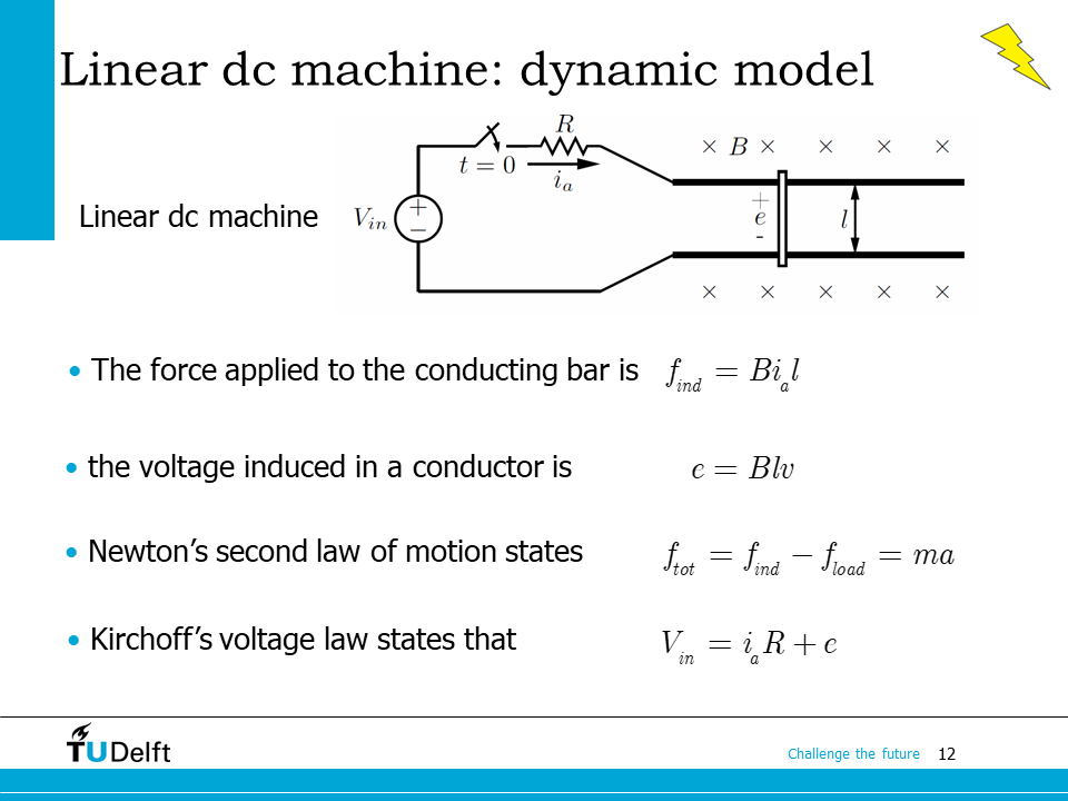
In the previous cases, we assume the conductor moves at a constant speed \(v\), here let us address the dynamic case where the conductor is accelerating at an acceleration \(a\).
The force applied on the conductor from the magnetic field is
where \(i_a\) is the current flowing in the conductor. We may also call it armature current. In electrical engineering, the word “armature” is used to name the part in an electrical machines to carry the force producing current.
The induced voltage in the conductor (armature) is
If the force exerted on the conductor from the load is \(f_{load}\), we are able to derive the mechanical dynamic equation
and from the electrical circuit, considering the circuit resistance \(R\) and the input voltage \(V_{in}\), we have the voltage equation
The above equations can be used to model and simulate the electromechanical dynamics of this simple linear machine.
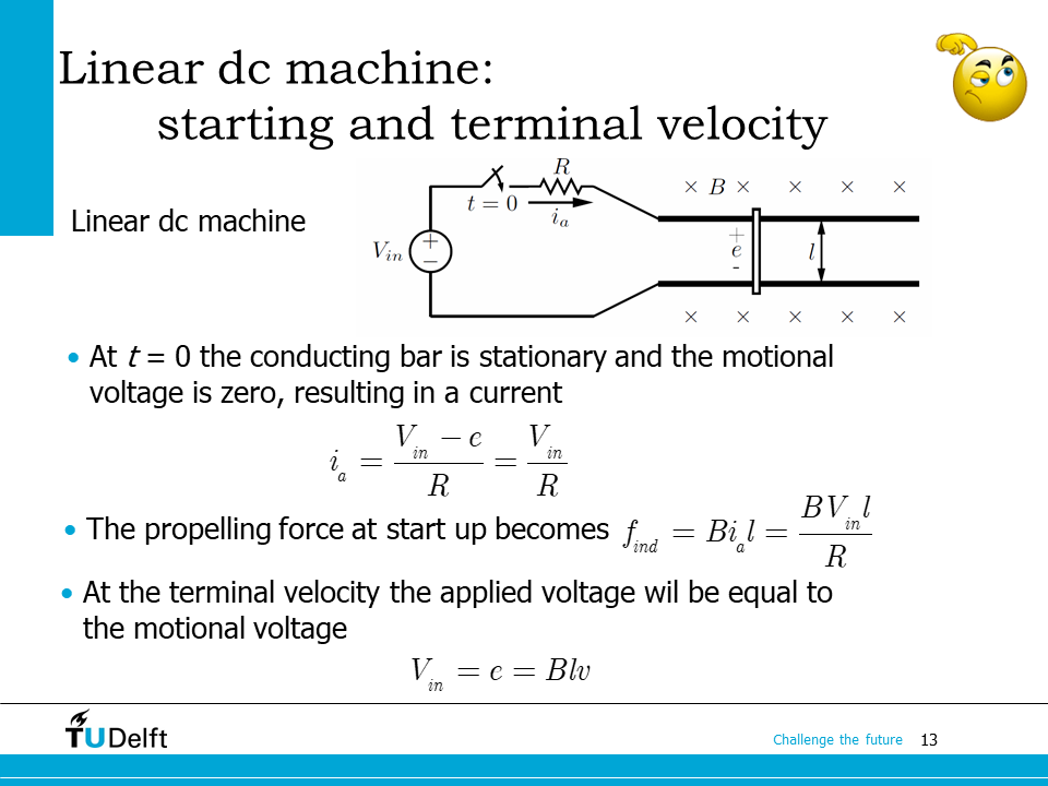
Now let’s use the dynamic equations derived above to calculate the starting force and the terminal speed of the conductor. When the conductor starts from standstill at \(t=0\), the induced voltage is not established yet because \(v=0\). The current reaches the maximum
The starting propulsion force will be \(f_{ind} = Bi_al = \frac{BV_{in}l}{R}\).
If we assume there is no load force, so \(f_{load} = 0\), and the rail is infinitely long, The conductor will be accelerating till the propulsion force reaches zero, i.e., the induced voltage becomes equal to the input voltage
So the terminal speed is \(V_{in}/(Bl)\).
This simple linear electric machine can be used as either an electric motor, which converts electrical energy into mechanical energy; or as a generator, which converts mechanical energy into electrical energy.
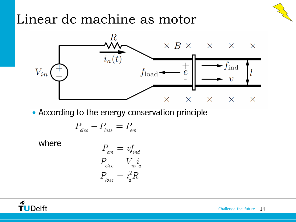
The motoring operation is described in the figure on this slide, be aware that the current \(i_a\) now flows into the induced voltage \(e\) during the motoring operation. Based on the energy conservation principle, we know
where \(P_{elec} = V_{in}i_a\) is the input electrical power, \(P_{loss} = i_a^2R\) is the loss caused by the resistance in the circuit, \(P_{em} = vf_{ind} = ei = Bliv\) is the electromagnetic power, which corresponds to the power which participates in the electromechanical energy conversion.
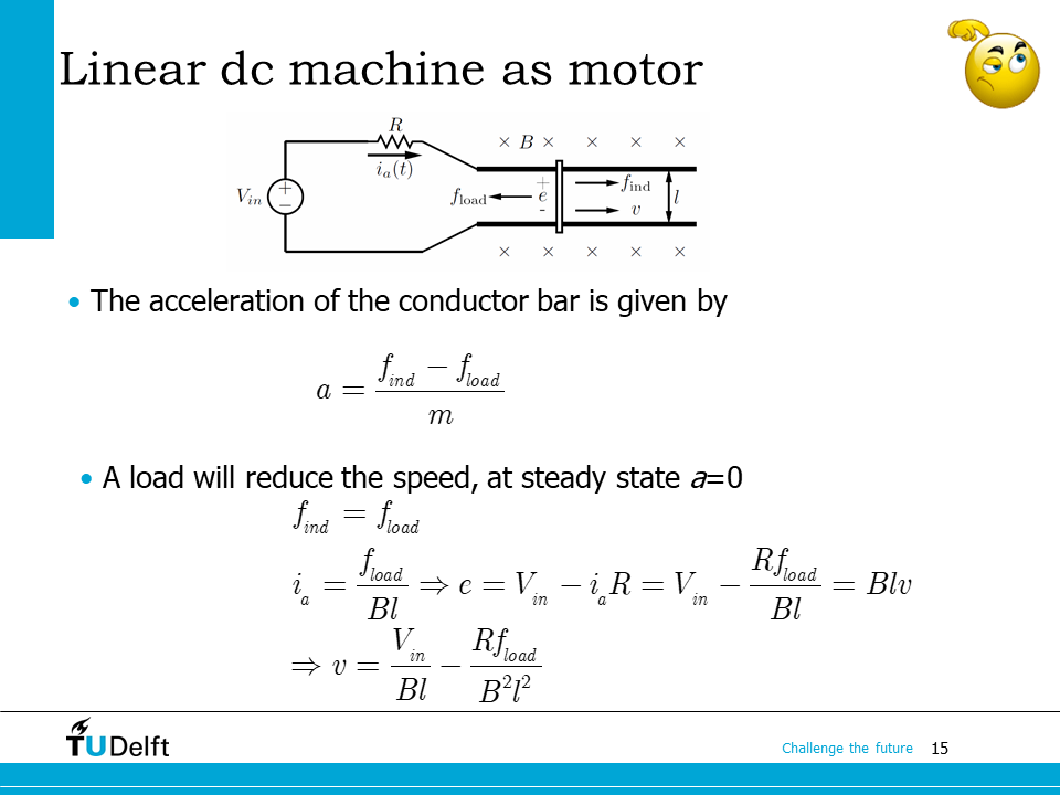
If there is a load force appears on the conductor, the acceleration stops when the electromagnetic force is balanced by the load force, i.e., \(f_{ind} = f_{load}\), so we have
We can see from the analysis above that the higher the input voltage, or the lower the load force, the higher the terminal velocity.
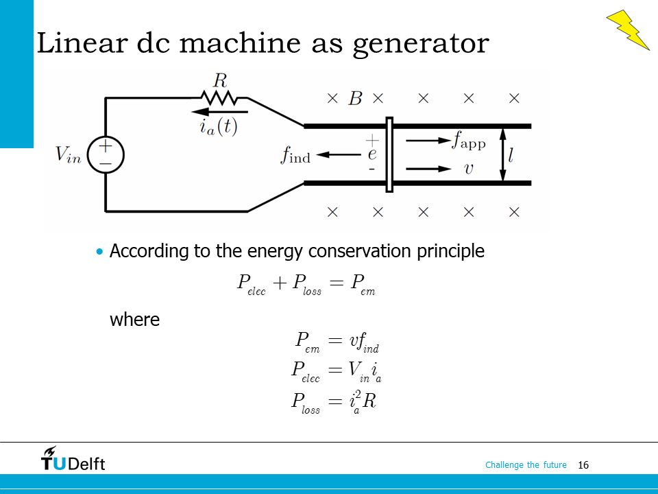
The figure on this slide shows the generating operation of the linear electric machine. An external force \(f_{app}\) is applied on the conductor in the direction of movement. The current now flows out of the induced voltage. The power flow revers its direction compared to the motoring case. Now the electromagnetic power \(P_{em}\) is not fully converted to the electrical terminal because of the loss, so we have
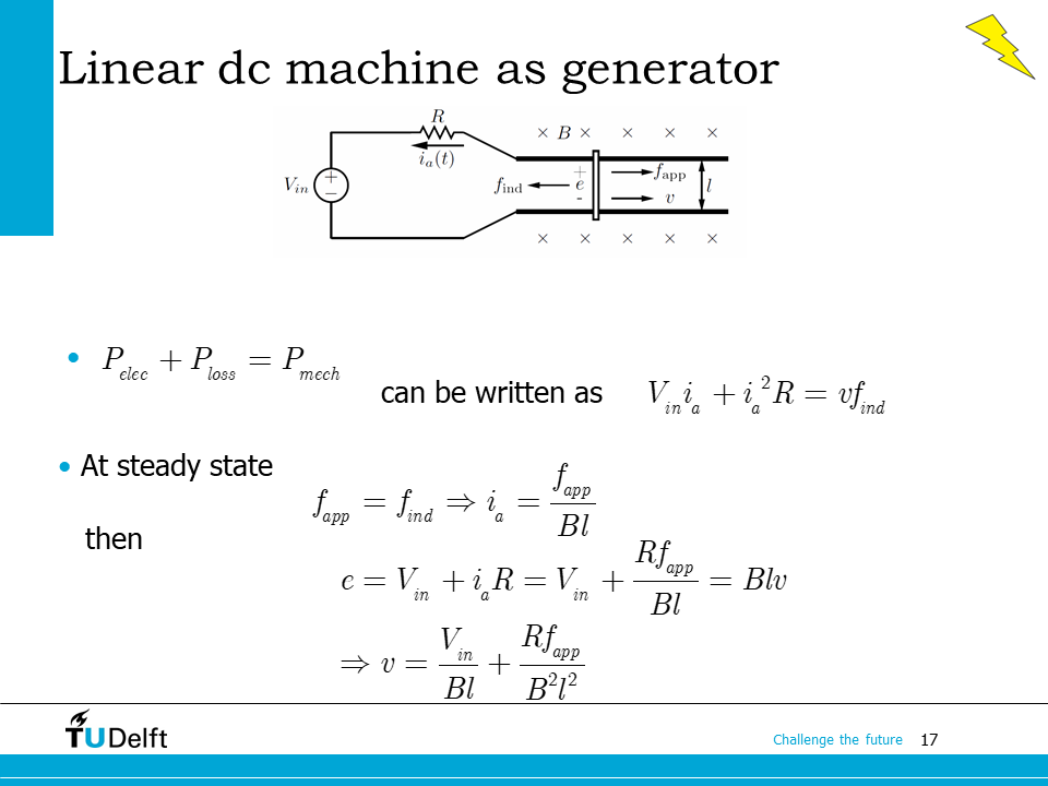
When this simple generator reaches steady state, the conductor stops acceleration, so \(f_{app}=f_{ind}\), based on the equations above, we have
Please pay attention to the positive current direction definition and the sign in the above equations.
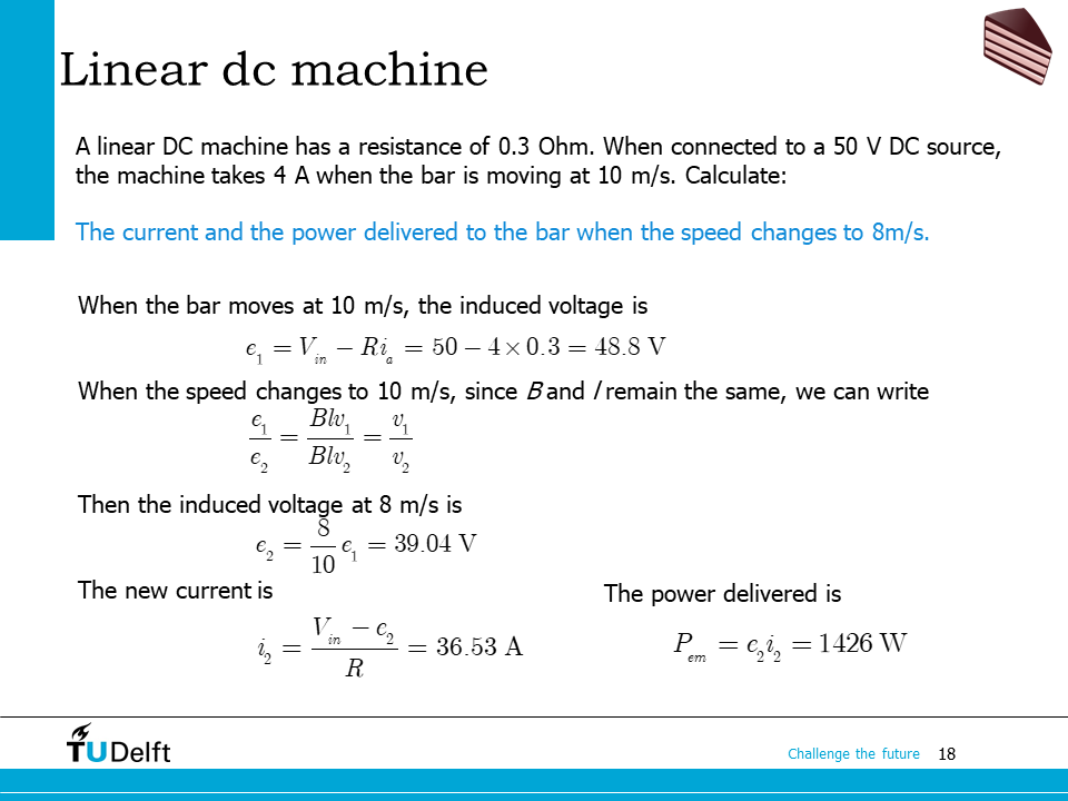
Now let’s practice what we have learned so far with the example on the slide. The Python script below gives the numeric solution
Show code cell source
R = 0.3
Vin = 50.0
Iin1 = 4.0
vbar1 = 10.0

# first calculate the induced voltage at 10m/s
e_1 = Vin - R*Iin1

# speed changes, induced voltage changes in proportion
vbar2 = 8.0
e_2   = vbar2/vbar1*e_1

# the current from Kirchhoff's Law
i_2 = (Vin-e_2)/R
# power delivered
p_em2 = e_2*i_2

print(f'The current in the bar at 8m/s is: {i_2:.3f} A.')
print(f'The power delivered to the bar at 8m/s is: {p_em2:.3f} W.')
The current in the bar at 8m/s is: 36.533 A.
The power delivered to the bar at 8m/s is: 1426.261 W.
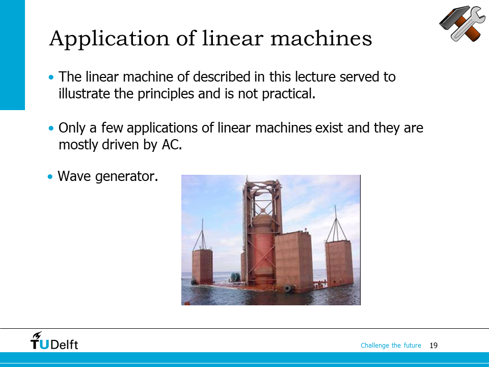
The linear electric machine example we show here help us illustrate the operation principle of electrical machines. But in practice, they have limited applications and are often driven by AC instead of DC.
On this slide, you can see a linear AC generator installed in the sea, which is used for generating electricity from waves. The generator was designed by a former colleague of mine, Henk Polinder, in the project Archimedes Wave Swing.
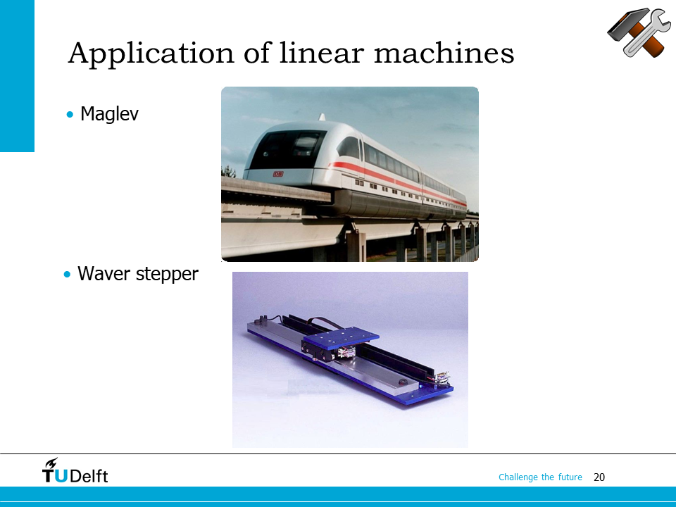
Other linear electric machine applications include high speed MagLev trains, and high precision wafer positioning system, as shown on the slide.
18.1. Simple electric motor 1: from linear to rotational#
In practice, rotational electrical machines are more extensively used. In this section, we will see how could we turn the simple linear machine to a rotational one.
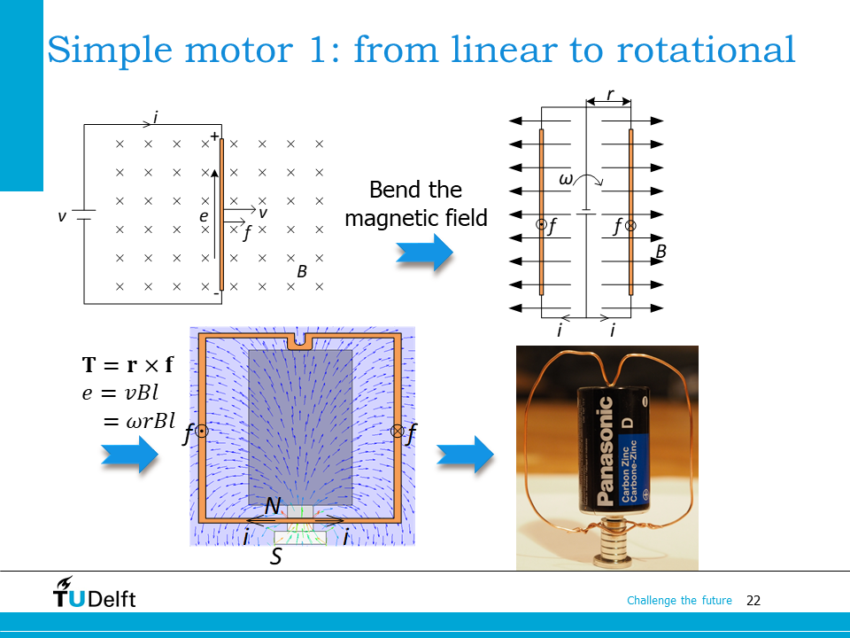
To enable a rotational motion, the direction of the electromagnetic force should change as the conductor rotates, so that is is always tangential to the moving direction. This could be achieved by first changing the direction of the magnetic field from into the screen, to the radially outspreading pattern as shown on the slide. To achieve a symmetric motion and balanced force, we could add another conductor on the other side of the power supply. By applying the right hand rule, we can see the electromagnetic force on the right conductor points into the screen, and that on the left conductor points out of the screen. The conductor pairs will rotate as a consequence of the two electromagnetic forces.
Recalling what we have learned in the mechanical system part of the course, the rotational machine can then be analysed better by torque, instead of force. The torque would be
where \(\mathbf{r}\) is the radius vector of the motion, \(F\) is the force. If the two are perpendicular to each other, the torque magnitude applied on one conductor is calculated as
The induced voltage is still \(e = Blv\), but \(v\) can be replaced with the rotational angular speed, so we have
In practice, such a simple rotational electric machine can be realised using several permanent magnets, a bare metal wire loop, and a battery. As you see on the slide, the simple machine construction is shown on the bottom right, while a magnetic field simulation is shown on the bottom left. You may try to implement this simple rotational electric machine at home and see whether it works.
18.2. Equivalent circuit#
It is more convenient to address the electrical mechanical energy conversion process using the concept of equivalent circuit.
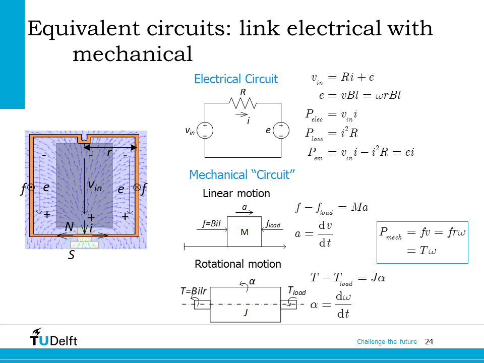
From the view point of the electrical, we can model the electrical machine system as an electrical circuit. In the equivalent circuit, the voltage source is connected to the induced voltage through a resistor which represents the Ohmic losses in the conductors. According to the Kirchhoff Law, we can write the equations below:
The input power, loss and converted electromagnetic power are
The above equations are valid when we follow he positive current direction as shown on the slide.
In the viewpoint of mechanical. We can draw the force diagram. According to Newton’s Law, the acceleration can be derived from the electromagnetic force, the load force and the mass, this is for linear motion. Tor rotational motion, the same thing can be done. However, the acceleration is replaced by angular acceleration and the mass is replaced by the moment of inertia here.
The electromagnetic power, which is equal to the mechanical power, becomes,
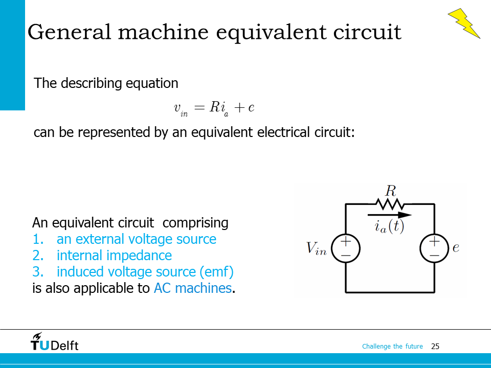
As we can see in the previous example, the steady state electrical performance of an electric machine can be represented by an equivalent electrical circuit.
The equivalent circuit of an electric machine comprises: i) an external voltage source to supply the machine; ii) an internal impedance of the electrical machine and iii) an induced voltage source, which is also called electromotive force.
The concept of equivalent circuit is applicable to not only DC machines we have studied so far, but also AC machines. Please be aware that the equivalent circuits are only used for steady state analysis. To analyse how electrical machines work during electrical or mechanical transients, we need to build up dynamic models using differential equations, which are out of the scope of the course.
18.3. Simple electric motor 2: how commutation works#
Now let us move on from the first simple motor to another more complicated one.
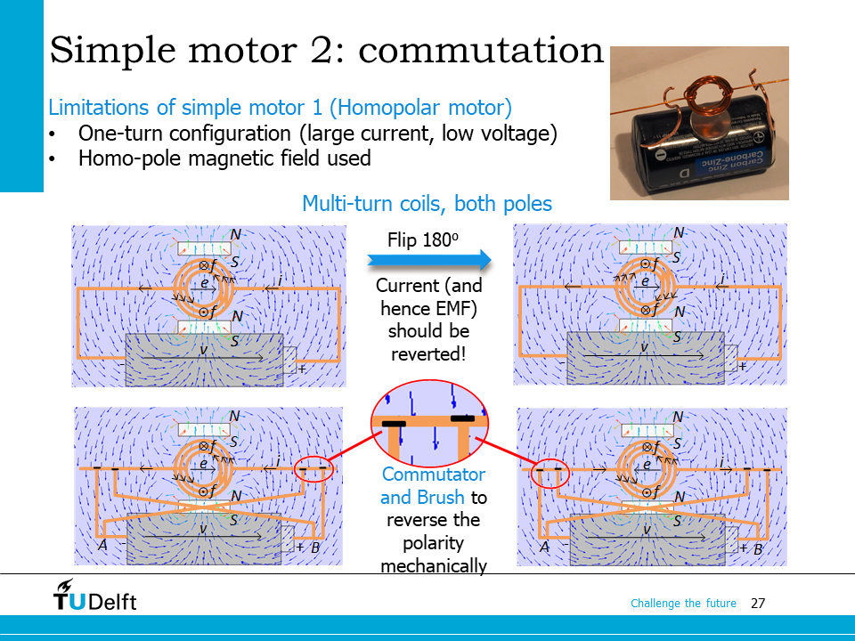
The simple motor we constructed just now has many drawbacks. The most fatal one is that it has a one-turn configuration, we can not add more turns into the coil. So if we want higher power ratings, we will meet a condition with rather low voltage and very large current. The large current will cut down the life of the conductors and generates extensive heat. Another drawback is that it only use one pole of the magnetic field, but not both. So this structure is rarely used for industry application.
Let us check what we can do to improve the machine for better feasibility. Firstly, we replace the single-turn coil by a multiple one. To keep the turns insulated from each other, enamelled wire is used here instead of the bare wires. Again, we put this coil into the filed generated by the magnets. And to improve the utilisation ratio, we introduce another magnet into the device. By connecting the coils to the battery, let us check what will happen in the next. In the first diagram, the current flow from the positive pole to the negative pole, and in the multiple turn coils, the current rotates counter-clockwise. By using the right hand rule, we can see that the forces on the upper conductors are perpendicular into the paper, and the forces on the lower conductors are perpendicular out of the paper. The coil will flip in this way by those force pairs. If the coil is flipped 180 degree, the current remain unchanged from positive to negative, however, the current in the coil now rotate clockwise. Using the right-hand rule, we will see that the force directions flip 180 degree too. The coil will flip in the opposite way. Hence is we do nothing else, the coil will flip back and forth.
Therefore, for continuous rotation, a switch that can reverse the current direction according to the rotation should be used. The switch should be operated automatically, not manually, otherwise the a human will work as the poor donkey as mentioned at the beginning of the lecture.
Luckily, some smart pioneers have come up with a very smart idea. We can introduce another circuit with the opposite direction into the device. And add insulation to shaft of the coils. As is indicated as the black segments. The upper part of the shaft is insulated from the forward circuit and the bottom part of the shaft is insulated from the backward circuit. As the coil rotates, the coil connects to the other circuit once flipped. We can check again by the right hand rule, we can see that now the force direction remain unchanged because the current and the coil are both flipped. We can call the coil shaft with insulation as commutators and the coil supporter as brushes. It is the commutator-brush system which makes the dc motor work.
Actually, the motor works too if we remove one pair of the brush and commutator and one magnet, due to the inertia of the coil. We can check it with the home-made motor on the top right of the slide. Look at the coil, the bottom part of the left coil shaft is tripped to provide half insulation. Put the coil on the brushes, we can see that the motor accelerates quickly. We use our learnt theory to build a motor with multiple turns successfully again. It is actually the simplest DC motors.
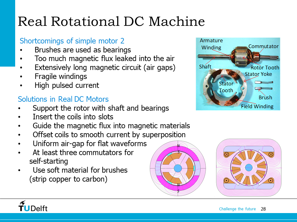
Although the previous DC machine based on the commutator-brush mechanisms is able to rotate continuously, it still has many drawbacks.
First, we use the brushes directly as shaft bearings, which is not robust enough. There is also too much magnetic flux leaked into the air, which is not contributed to electromechanical energy conversion. The magnetic circuit is also very long, i.e., the reluctance is too large. The windings are fragile and not protected from mechanical stresses. As the coil rotates, the coil also sees pulsating voltages, which makes both current and torque ripples.
To solve the previously mentioned problems, in practical DC machines, we take many measures to make it more robust, efficient and compact, as noted on the slide.
On the right hand side of the slide, you can see an anatomy of the real DC machine and the simulated magnetic flux lines inside it. As you can see, the coils are now embedded in slots punched on magnetic cores. The air-gap between the rotor and the stator is very small. In the two magnetic flux line plots, the left one shows a permanent magnet DC machine, where the field is excited by permanent magnets; the one of the right is a wound field DC machine, where the field is excited by current in the field coils. We will study both of them in the coming lectures.
That’s the end of the introduction to electrical machines. If you are curious about the early stage work of engineers and scientists to make electrical machines possible and more and more efficient, you may check this link to learn the history of electrical machines.
In the coming three lectures, we will learn the DC machine construction, analysis of DC machines based on equivalent circuits and how to control them using DC drives.