DC Machines

19. DC Machines#

In this lecture we will learn how voltage and torque is continuously generated in an DC machine, the construction of the DC machines and what the motivations are to construct them in the current way.

19.1. General electrical machine principle and construction#

Let’s first review the general operation principle of electrical machines.

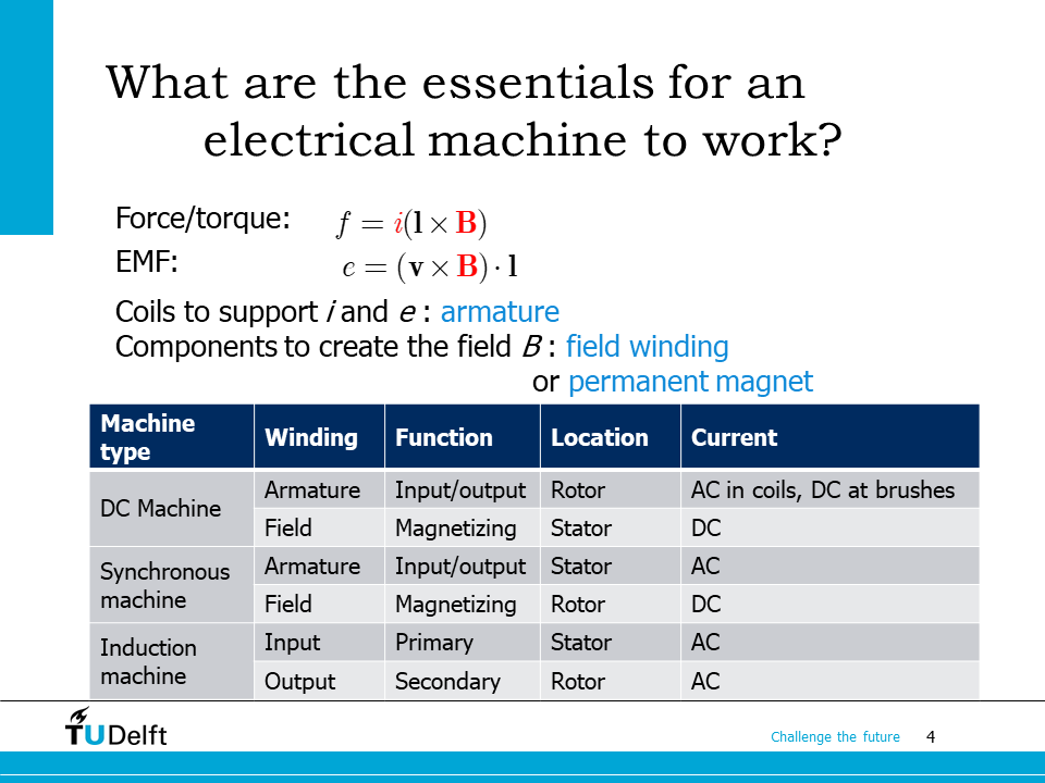
As we have learnt in the previous lecture, we know the operation of the electrical machines relies on Faraday’s law of induction and Lorenz’s force. From the two laws, we know in order to make the electrical machine work, we need both electrical current and magnetic field. Therefore, in the construction of an electrical machine, we need the coils to support the torque/force generation current \(i\) and the induced voltage \(e\), and the components to create and convey the magnetic field \(B\).

The component to support the torque/force generation current \(i\) and the induced voltage \(e\) is also called armature.

In practice, we can create the magnetic field from either current flowing in a winding (field winding) based on Ampere’s law, or from permanent magnets.

Depending on where the induced voltage is generated and where the field is generated, we can classify the electrical machine into three main categories.

DC machine#: The armature is on the rotor side, while the magnetic field is generated from the stator. The armature winding bears AC currents, but it is mechanically rectified to DC via the commutator-brush mechanism as we have shown in the last lecture and will investigate in detail later in this lecture.
Synchronous machine#: The armature is on the stator side, where AC induced voltage is generated and AC current flows. The field winding is placed on the rotor, which flows DC current.
Induction machine#: The current on both stator and rotor sides are AC. At standstill, the induction machine operates as a transformer with air-gap. As rotor rotates, a current with slip frequency (the difference between the stator supply frequency and the rotor rotating frequency) flows in the rotor winding.

In this lecture, we will first analyse the DC machine in detail.

19.2. Single loop coil with commutator#

Let us start the analysis from one single loop of armature coil inside an DC machine.

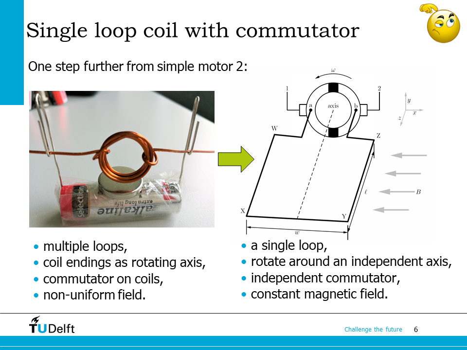
In contrast to the simple motor we made in the last lecture, we assume there is only one loop of wire to form the coil, which rotates around an axis independent from the coil. The commutator and brushes are attached to the end of the coil loop, as shown on the right hand side. The magnetic field is assumed to be constant, and pointing leftwards horizontally (negative x direction).

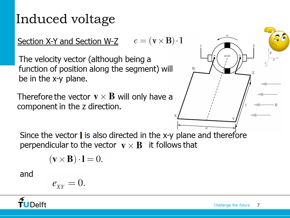
The coil loop comprises of four sections, let us first analyse the X-Y and W-Z sections. The induced voltage in the segments can be calculated from Faraday’s law, which is \( e = (\mathbf{v}\times\mathbf{B})\cdot \mathbf{l} \).

Since the axis is aligned to the z-axis, \(\mathbf{v}\) is always in the x-y plane, and \(\mathbf{B}\) is in the negative x direction, the vector \(\mathbf{v} \times \mathbf{B}\) will only have a component in the z direction.

Since \(\mathbf{l}\) is also directed in the x-y plane for the two segments, therefore, \(\mathbf{v} \times \mathbf{B}\) and \(\mathbf{l}\) are always perpendicular to each other, so the induced voltage

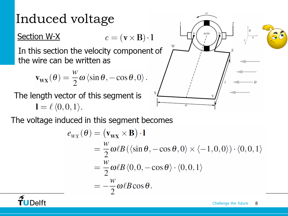
\[ e_{XY} = e_{WZ} = (\mathbf{v}\times\mathbf{B})\cdot \mathbf{l} = 0. \]

Then let us analyse the W-X section. As the coil loop rotates, the angle formed by the coil plane and the xz plan is defined as \(\theta\). So the velocity of the W-X section is derived as

\[ \mathbf{V_{WX}}(\theta) = \frac{w}{2}\omega <\sin\theta, -\cos\theta, 0>. \]

Substitute the above equation, \(\mathbf{l} = <0, 0, l>\) and \(\mathbf{B} =<-B, 0, 0>\) into the induced voltage equation we have

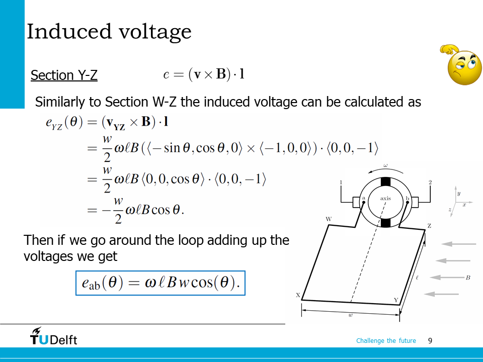
\[\begin{split} \begin{align} e_{WX}(\theta) &= (\mathbf{V_{WX}}\times \mathbf{B})\cdot \mathbf{l} \\ &= \frac{w}{2}\omega lB<0,0,-\cos \theta>\cdot <0,0,1> \\ &= -\frac{w}{2}\omega lB\cos\theta. \end{align} \end{split}\]

Similarly for the Y-Z section, the velocity is

\[ \mathbf{V_{YZ}}(\theta) = \frac{w}{2}\omega <-\sin\theta, \cos\theta, 0>. \]

and the length vector is

\[ \mathbf{l} = \mathbf{l} = <0, 0, -l>. \]

So we have

\[\begin{split} \begin{align} e_{YZ}(\theta) &= (\mathbf{V_{YZ}}\times \mathbf{B})\cdot \mathbf{l} \\ &= \frac{w}{2}\omega lB<0,0, \cos -\theta>\cdot <0,0,-1> \\ &= -\frac{w}{2}\omega lB\cos\theta. \end{align} \end{split}\]

Then the total induced voltage along the WXYZ coil loop seen from the terminal ab is

\[ e_{ab}(\theta) = \omega lBw\cos(\theta). \]

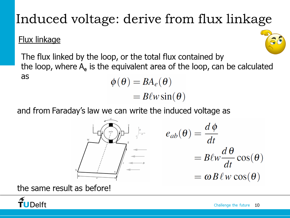
The analysis in the previous two slides can also be derived from the flux linkage.

The flux linked by the loop is \(\phi(\theta) = \int_A \mathbf{B} \cdot \mathrm{d} \mathbf{A}\), which can be derived as the constant flux density \(B\) multiplied by the equivalent area of the loop \(A_e(\theta) = lw\sin(\theta)\). So we have

\[ \phi(\theta) = BA_e(\theta) = Blw\sin(\theta). \]

From Farday’s law, we know the total induced voltage along the WXYZ coil loop seen from the terminal ab is

\[ e_{ab}(\theta) = \frac{\mathrm{d}\phi}{\mathrm{d} t} = \omega Blw \cos(\theta), \]

which is the same as we derived based on \( e = (\mathbf{v}\times\mathbf{B})\cdot \mathbf{l} \).

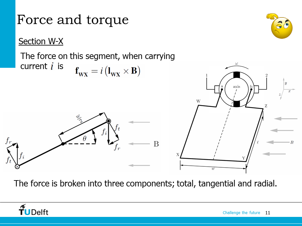
Then let us calculate the torque applied on the coil by the electromagnetic force. We start with the W-X section. Applying Lorenz’s law, we have

\[ \mathbf{f_{WX}} = i (\mathbf{l_{WX}}\times B). \]

The force can be divided into its tangential and radial component, and only the tangential force produces torque.

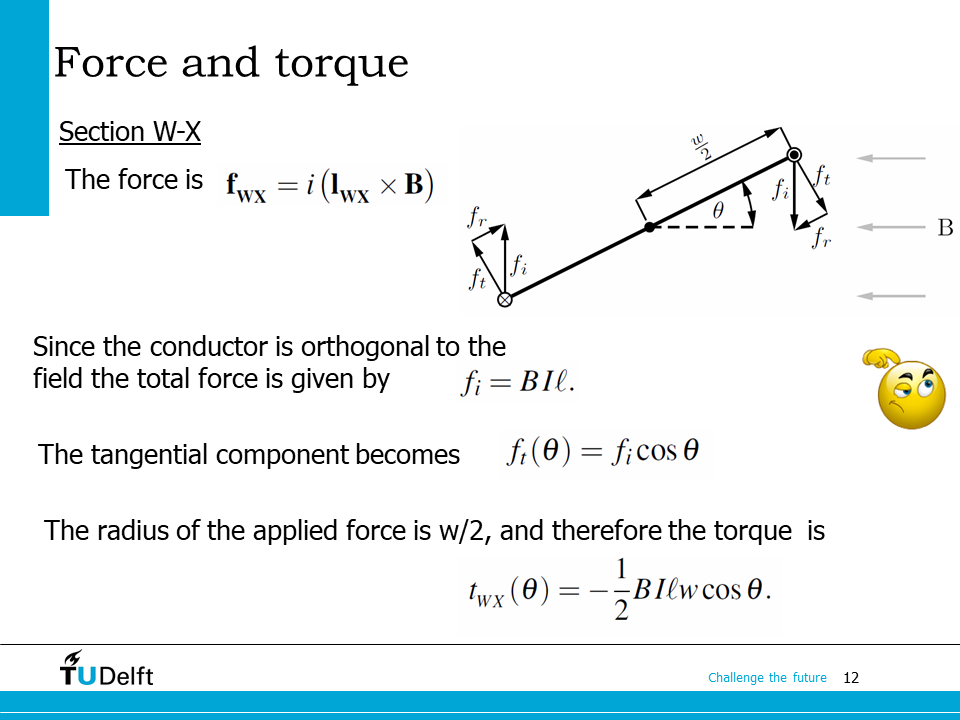
The total force on the W-X segment is \(f_i = Bil\) since \(\mathbf{l}\) and is perpendicular to both \(\mathbf{l}\) and the flux density vector \(\mathbf{B}\). Therefore, the tangential force component is

\[ f_t(\theta) = Bil\cos(\theta). \]

The torque produced by it is

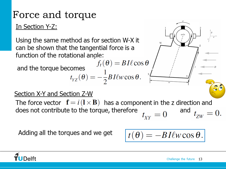
\[ t_{wx} = f_t(\theta) \frac{w}{2} = -\frac{w}{2}Bil\cos(\theta). \]

For section Y-Z, similar analysis can be done, which gives the torque

\[ t_{yz} = f_t(\theta) \frac{w}{2} = -\frac{w}{2}Bil\cos(\theta). \]

For section X-Y and Z-W, the force is always in the z direction because both \(\mathbf{l}\) and \(\mathbf{B}\) are in the XY plane, so the generated torque with respect to the axis is zero.

Adding all the torques applied on the the coil loop, we have the total torque

\[ t_{\theta} = -wBil\cos(\theta). \]

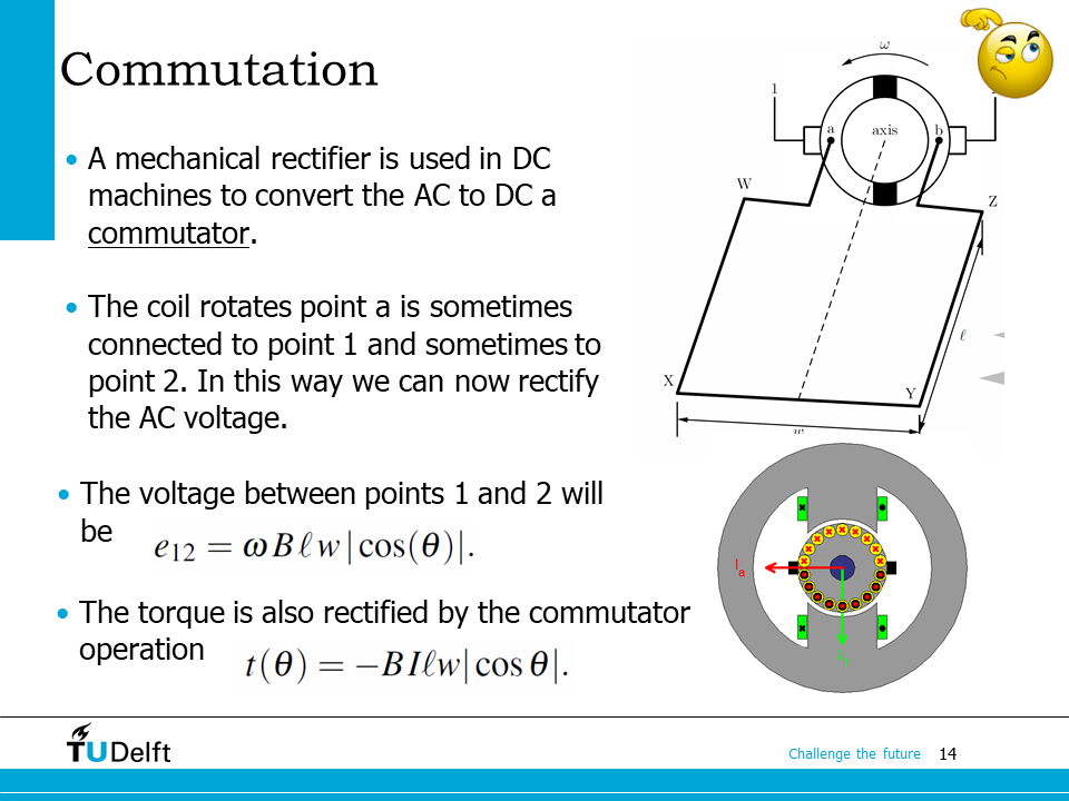
Now we see if the current in the coil \(i\) has a fixed value, both the induced voltage and the torque will be alternating. Thanks to the commutator-brush mechanism as we explained in the last lecture using the simple machine, as the coil rotates, point a is sometimes connected to point 1 and sometimes to point 2. In this way we can now rectify the AC voltage, so that at the brushes, we have the “mechanically rectified” DC induced voltage

\[ e_{12} = \omega Blw |\cos(\theta)|. \]

Similarly, the current in the coil also alternates because of the commutator-brush mechanism, so the torque is also rectified, we have

\[ t_{\theta} = -wBil|\cos(\theta)|. \]

As we can see, although we see DC voltage and current at the brushes of the DC machine, before the commutator, the current and voltage inside the coil of the DC machine are alternating.

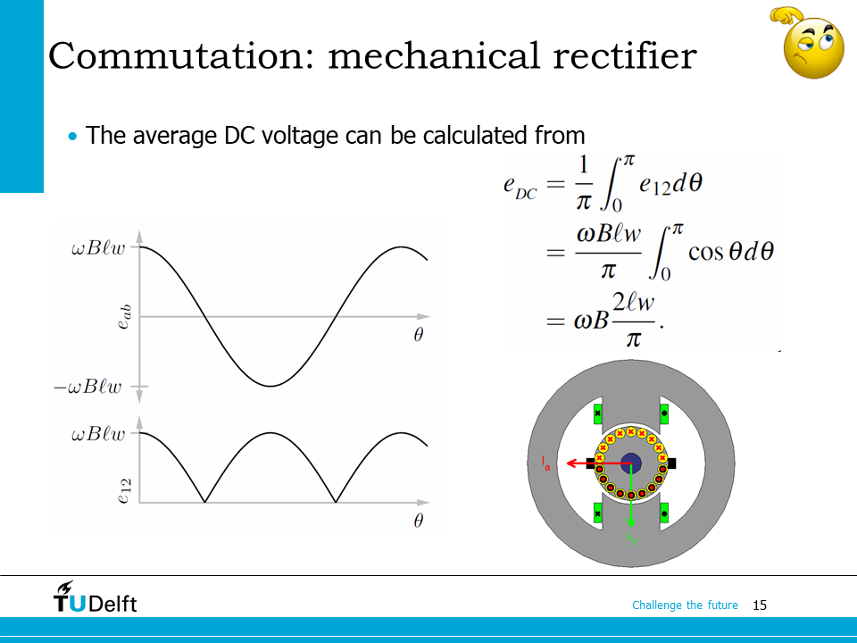
The average induced voltage after rectification of the commutator-brush mechanism is

\[\begin{split} \begin{align} e_{DC} &= \frac{1}{\pi}\int_0^{\pi} e_{12}\mathrm{d}\theta \\ &= \frac{\omega l B w}{\pi}\int_0^{\pi} \cos\theta\mathrm{d} \theta \\ &= \omega B \frac{2 l w}{\pi}. \end{align} \end{split}\]

Similarly, the average torque is \(t_{av} = -Bi \frac{2 l w}{\pi} \).

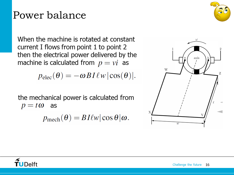
From the torque and induced voltage equations, it is easy to see that the power is still balanced: the electromagnetic power is equal to the mechanical power.

19.3. Upgrade the simple DC machine#

Then we could upgrade the one loop case to a DC machine in practice.

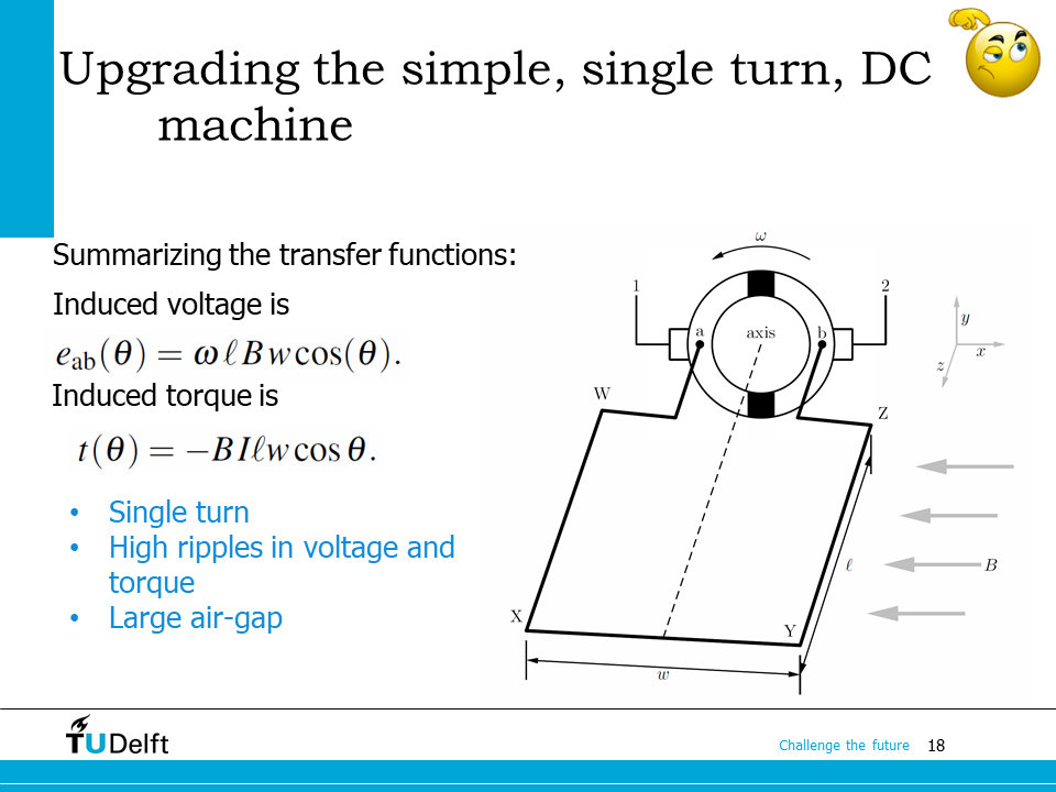
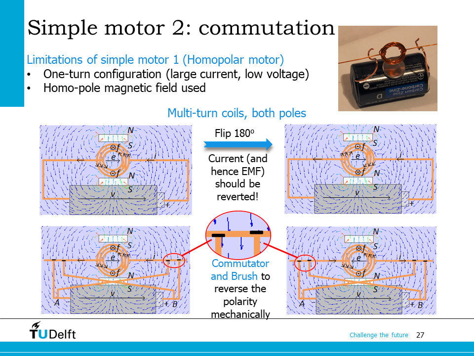
The single-loop DC machine has high voltage, current and torque ripples, and large air-gap. More practical construction is needed to solve the problems.

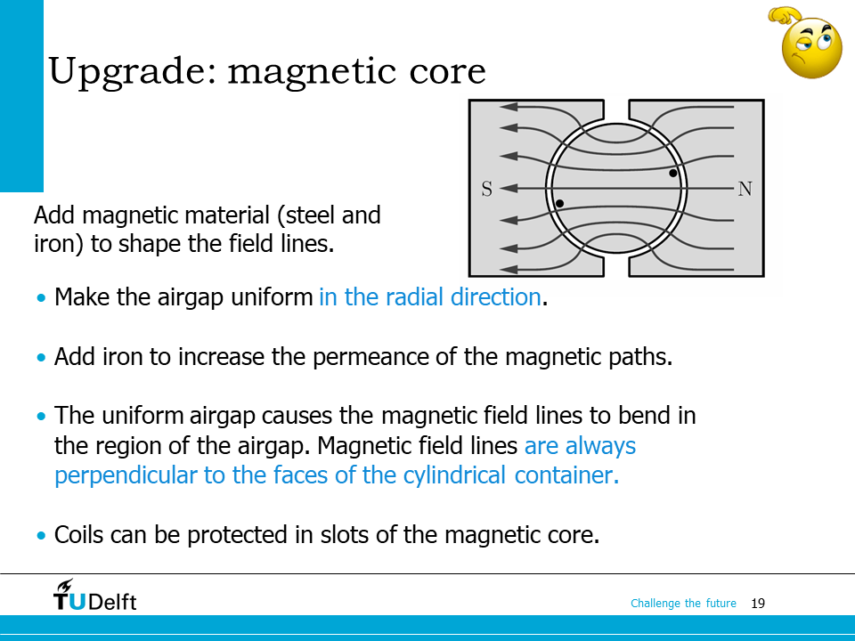
In realistic DC machines, in order to make them more efficient and more ripple free, we add magnetic cores to the rotor and the stator. As we can see on the slides, magnetic poles are formed by the stator core, and a round rotor is placed between inside the poles. A uniform circular air-gap in the radial direction is shaped by the stator and the rotor. Magnetic cores will shape the magnetic flux lines, so that they are always perpendicular to the surfaces of the cylindrical rotor and the stator pole faces, apart from the interpole regions at \(\theta = 90^\circ\) and \(\theta = 170^\circ\). The radial flux density waveform in the air-gap is therefore becomes flat-shaped.

By adding the magnetic core, the magnetic permeance of the magnetic circuit is also increased significantly, therefore, we will need much less field current to excite the same \(B\) (Ampere’s law). Another advantage of adding the magnetic core is now coils can be embedded inside the slots punched on the magnetic core. This way the coils are better protected.

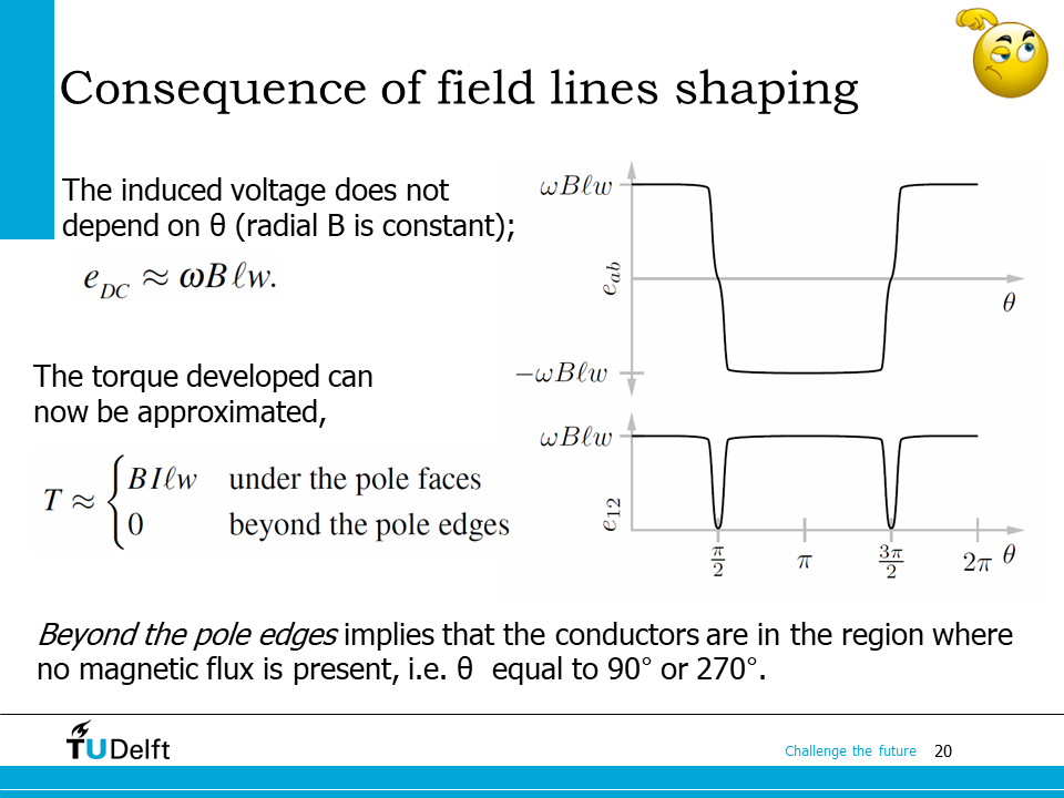
As we can see from the \(B\) waveform on the slide, the flat-topped radial flux density will lead to a constant induced voltage when the coil conductors are below the pole faces, i.e., \(e_{DC} = \omega Blw\), the torque is also contant \(T = Bliw\).

When the coil conductors are beyond the pole edges, or are under interpoles around \(\theta = 90^\circ\) or \(\theta = 270^\circ\), the induced voltage and the torque can be considered to be zero because of the sudden drop of flux density in interpoles.

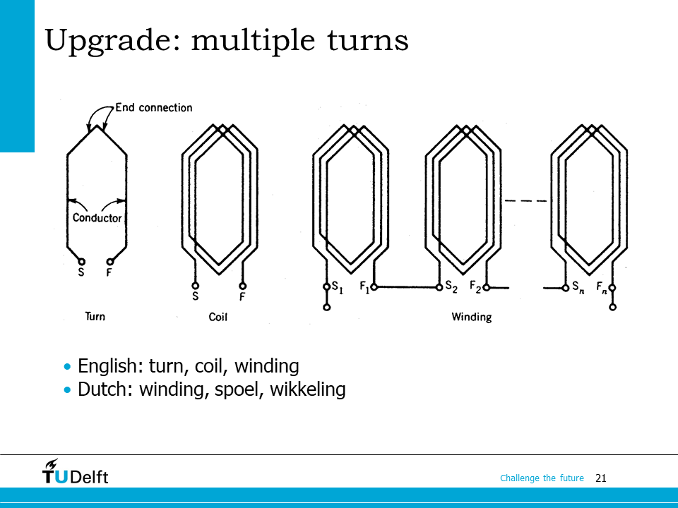
In practice, to eliminate the sudden drop in torque and induced voltage, we usually use multiple armature coils spreading along the rotor cylinder to form an armature winding. And to increase the induced voltage, so that less current is needed, we may use multiple coil loops for form a single coil. Each coil loop is called a turn. Therefore, the basic unit for a machine winding is a turn. Multiple turns make a coil, and multiple coils make a winding. To form a winding from multiple coils, we could connect them in series, in parallel, or in a hybrid way, depending on the type of electrical machine and the electrical requirements.

Similarly, we may have more than 2 poles in the DC machine, each pole has its field coil, and all the coils are inter-connected in series or in parallel to form the field winding.

Note

In English the three components are called English: turn, coil and winding respectively. However, in Dutch they are called winding, spoel, wikkeling respectively. A “winding” in Dutch is actually a “turn” in English.

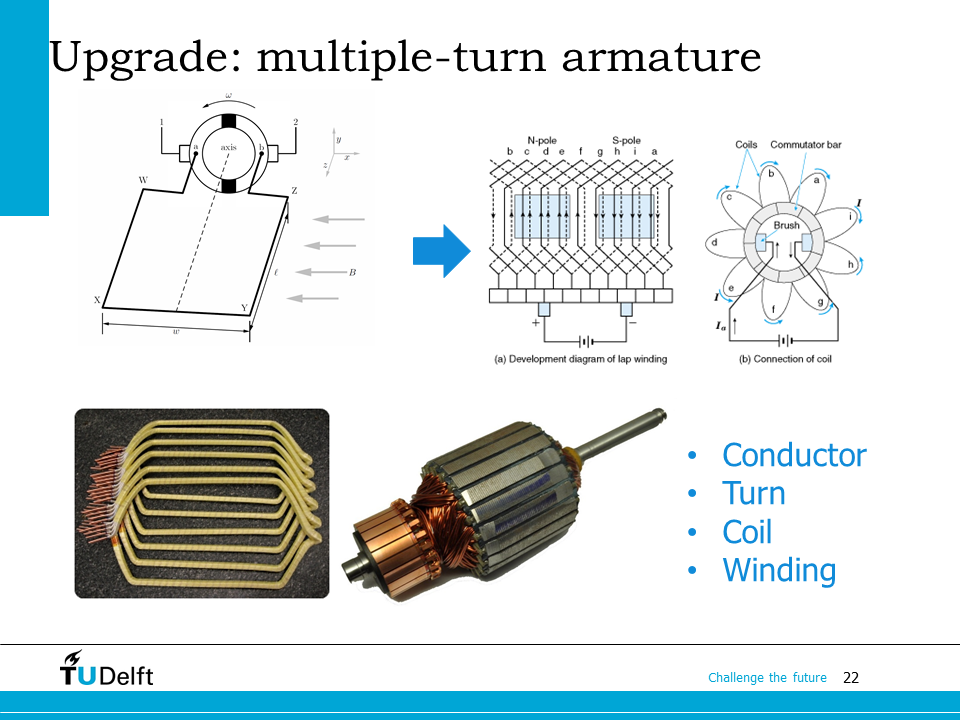
This slide shows how a realistic DC machine is constructed in practice by using a multiple-coil armature winding and attaching the ends of each coil to the commutators. As the rotor rotates, the coils are conducting from one to another, to produce a smoother torque and induced voltage.

This animation may help you understand how a multiple-coil DC machine armature winding commutates from one to another.

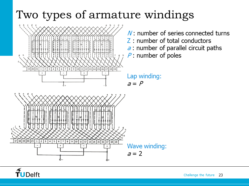
There are mainly two ways to attach the armature coil terminals to the commutators to make the armature winding.

Lap winding#: As shown in the top figure, each coil overlaps the next so that there are as many armature current paths through the machine as there are magnetic poles on the machine. So if \(a\) is the number of parallel circuit paths in the armature, \(P\) is the number of poles, we have \(a=P\) for lap winding.
Wave winding#: The wave winding is also called the series winding. As shown in the bottom figure, the coils follow each other on the surface of the armature in the form of waves, so that there are two current paths in parallel. Therefore, for a wave winding \(a=2\).

Obviously, the lap winding is more suitable for low voltage high current applications and the wave winding is more suitable for high voltage, low current applications.

19.4. Machine constant#

Having understood the operation principles, now let us study the quantitative way to analyse the DC machine performance.

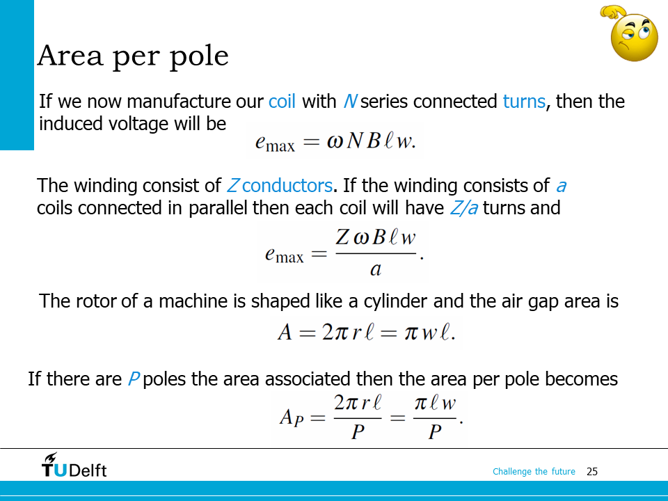
From previous analysis we know if there are \(N\) turns connected in series, the total induced voltage will be \(e_{max} = \omega NBlw\). The number of turns in series \(N\) can be obtained from the total conductors in all armature slots \(Z\), divided by the number of parallel paths \(a\), so

\[ e_{max} = \frac{Z\omega Blw}{a}, \]

where \(w = 2r\) is the width of the coil span.

The total surface area of the armature cylinder is \(A = 2\pi r l = \pi w l\). The surface area per magnetic pole is \(A_p = A/P = \frac{\pi l w}{P}\).

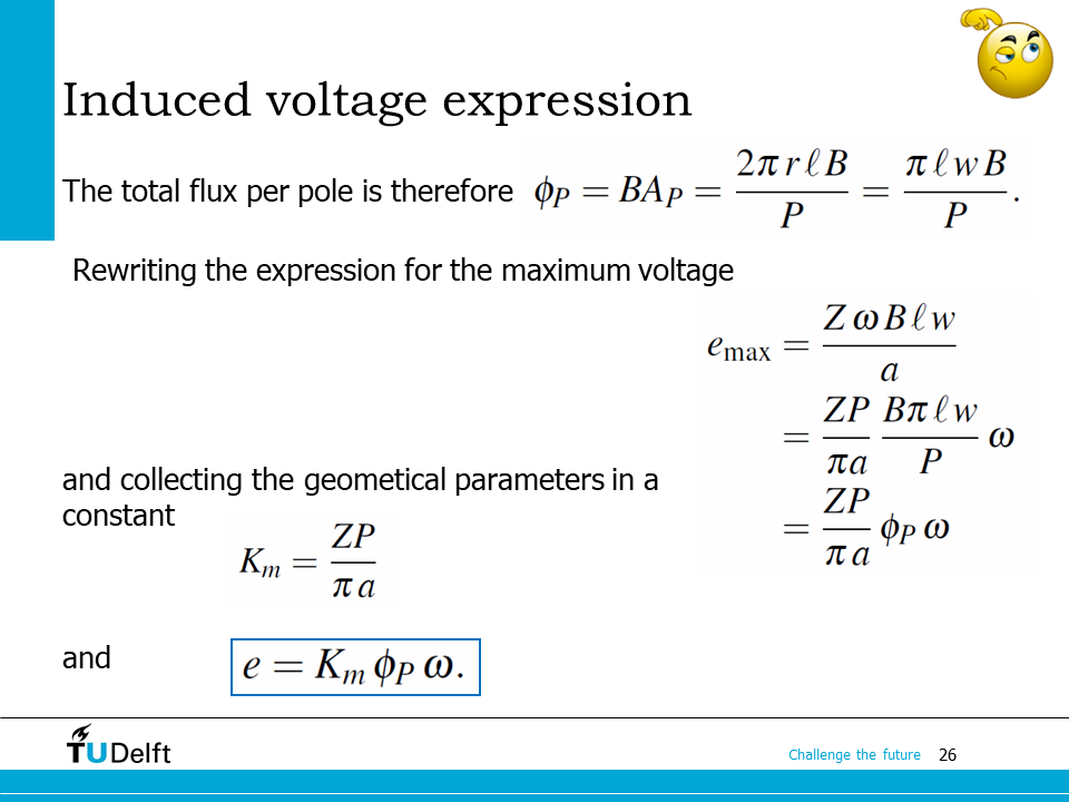
From the area per pole and the flux density, by assuming the flux density is always perpendicular to the cylindrical surface of the armature, the flux per pole is derived

\[ \phi_P = BA_P = \frac{2\pi rl B}{P} = \frac{\pi l w B}{P}. \]

It takes a time of \(\mathrm{d} t = 2\pi/(P\omega)\) for the armature rotates from one magnetic pole to the next one. During this time interval, the flux linkage changes by

\[ \mathrm{d}\lambda = N[\phi_P - (-\phi_P)] = 2N\phi_P. \]

Based on Faraday’s law, the induced voltage is

\[\begin{split} \begin{align} e_{max} &= \frac{\mathrm{d}\lambda}{\mathrm{d}t} \\ &= \frac{2N\phi_P}{2\pi/(P\omega)} \\ &= \frac{NP}{\pi}\phi_P\omega \\ &= \frac{ZP}{\pi a}\phi_P\omega. \end{align} \end{split}\]

If we collect all geometrical parameters in the equation above, and name it as the machine constant \(k_m\), we have

\[ K_m = \frac{ZP}{\pi a}. \]

and

\[ e = K_m\phi_P \omega. \]

Here the derivation is done based on \(e = \mathrm{d} \lambda /\mathrm{d} t\), which gives us the same results as the derivation based on \(e=Blv\) shown on the slide. It is easy to derive that the machine constant is a dimensionless constant.

On this slide, the total torque is derived by summing up the torque applied on all series connected turns. We may also derive it from the power balance. The electromagnetic power is \(P_{em} = eI = K_m\phi_P\omega I\), which is equal to the mechanical power delivered by the DC machine,

\[ P_{mec} = T\omega = P_{em} = K_m\phi_P\omega I, \]

so we have

\[ T = K_m \phi_P I. \]

As you can see, the machine constant \(K_m\) bridges the electrical circuit and the mechanical system for the DC machine.

19.5. Real DC machine construction#

Now let us see some realistic DC machine constructions to learn how a real DC machine looks like.

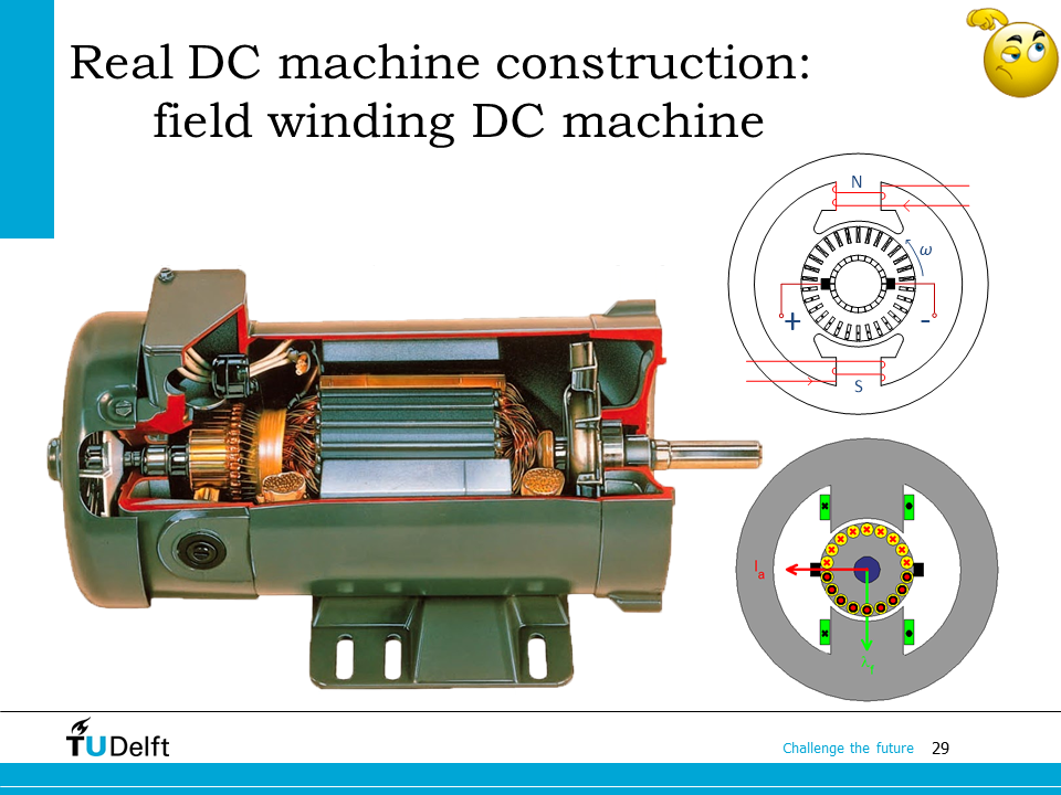
What you see on the slide is a wound field DC machine or field winding DC machine, where two big coils on the stator side is used to excite magnetic field. On its right side, a schematic is made to show its construction.

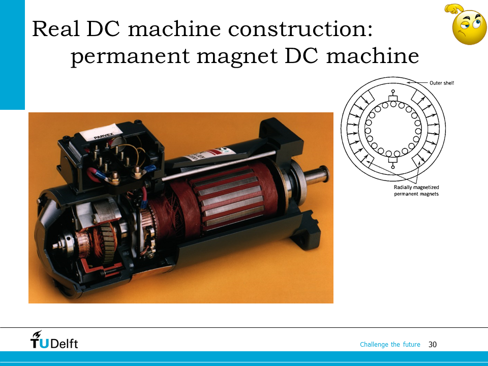
Here what you see is a permanent magnet DC machine, inside which the magnetic field is generated from the permanent magnets mounted on the inner wall of the stator. You may also see there is another small DC machine attached to the same shaft on the left. It is a tachogenerator used to measure the rotational speed. The faster the machine rotates, the larger the induced voltage is measured from the tachogenerator. Therefore, we convert the speed signal to electrical signal, which makes it easier for us to control the speed of the machine electronically.

The home work below is for you to practice what we learn today. After taking the lecture, you should be able to distinguish the motoring and generating operation modes, and use the machine constant to solve similar questions.

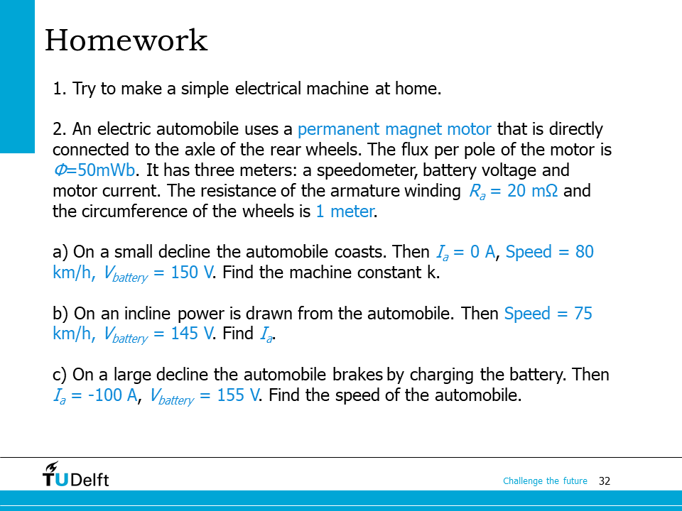
Please try to solve the homework by yourself. You may click and check the code below to check your answers.

Note

Pay attention to whether the motor notation or the generator notation is used when solving electrical machine problems. In the two notations, the positive direction of the current is different.

a) The machine constant is 21.486.
b) The machine constant is 218.750 A.
c) The speed of the automobile is 23.259 m/s or 83.733 km/h.