15. Coupled Coils#
Based on the magnetic principles and magnetic circuit approach we studied in the last lecture, here we will extend their applications to more complicated cases, and deal with the case with air gap. Then we will use an example to show saturation in magnetic materials. In the end, coupled coils and ideal transformers will be studied.
15.1. Square core inductor#
Let us first analyse a square core inductor, which is a bit more complicated than the toroidal one as we studied in the last lecture.
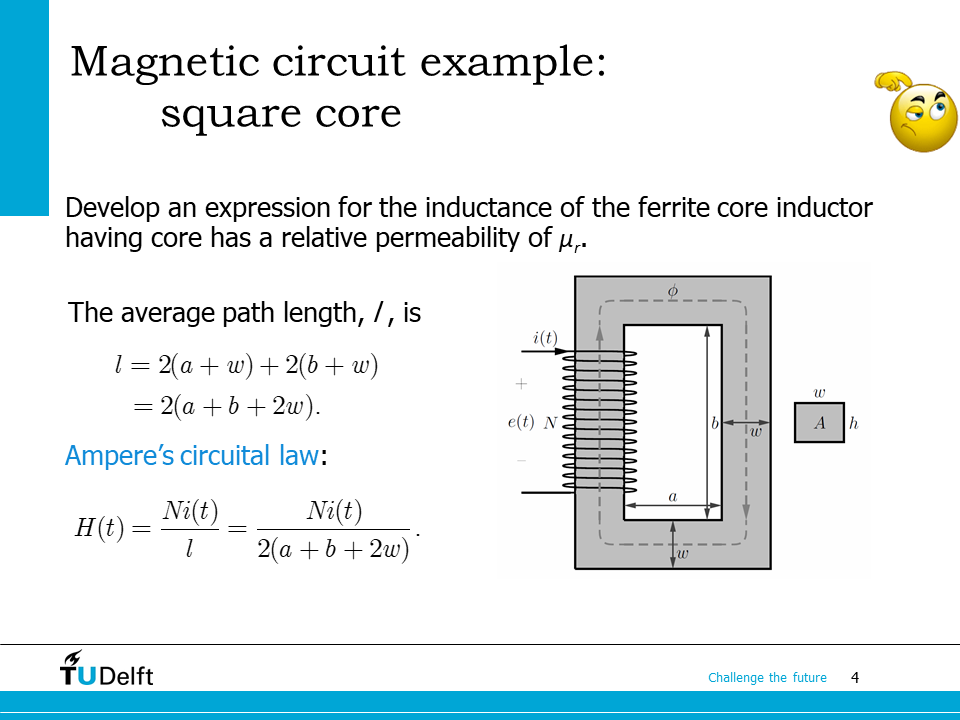
Based on the geometry of the magnetic core, the average length of the magnetic path is measured in dashed loop in the centre of the core frames, therefore we have
Similarly the area is \(A = wh\).
Based on the Ampere’s circuital law, we have
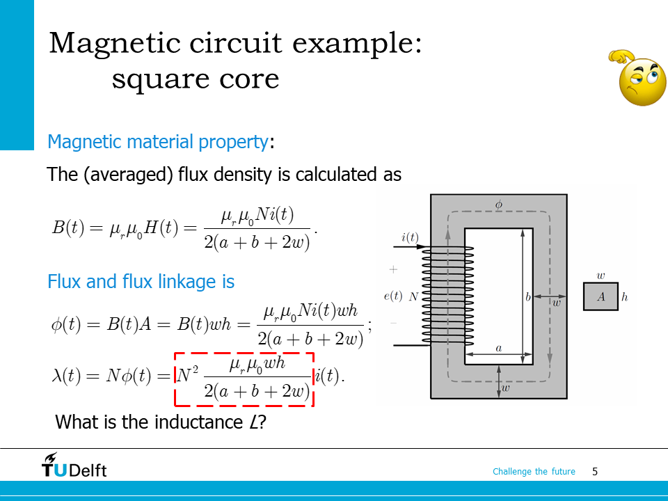
Flux density \(B\) is solved from the material property. The relative permeability of the core material is \(\mu_r\), so we have
The magnetic flux and flux linkage of the coil can then be solved as shown on the slide.
Alternatively, we can solve the problem using magnetic circuit.
The magnetic circuit reluctance is
The magnetic flux is
The flux linkage is
Since \(e(t) = \frac{\mathrm{d} \lambda(t)}{\mathrm{d} t} = L \frac{\mathrm{d} i(t)}{\mathrm{d} t}\), we can see here
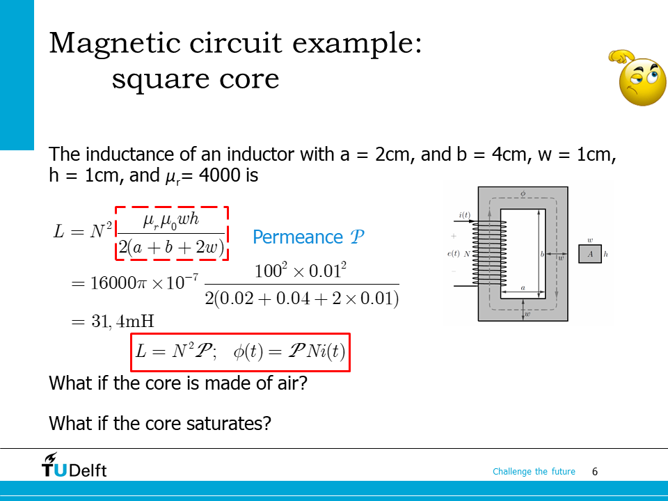
The inductance expression here is exactly \(N^2 \mathcal{P}\), where \(\mathcal{P}\) is the magnetic permeance of the magnetic circuit.
Substituting the parameters in, we are able to solve the numerical value of the inductance.
From the example above, we can conclude, in general for a single inductor, we have
and
As we can see here, the inductance is proportional to the permeance of the magnetic core, which is determined by the geometry and the permeability of the core. If air is used instead of ferromagnetic material for the core, the inductance will drop significantly. However, on the other hand, ferromagnetic material is prone to saturation, which will reduce the permeability when the flux density is higher than the saturation flux \(B_s\).
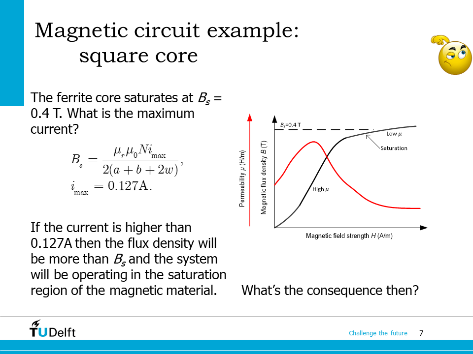
Let us use this example to see how saturation limits the maximum operation current. If the core saturates at \(B_s = 0.4~\mathrm{T}\), based on the flux density expression we derived above, we can see the maximum allowable current so that the core operates below saturation is calculated as
If the current through the inductor is larger than this value, the permeability will drop significantly, the inductance will drop accordingly.
15.2. Toroidal core inductor with air gap#
The previous two inductors have homogeneous magnetic cores, i.e., there is no discontinuity in core material. Now let us study the case where the magnetic core is interrupted by an air gap.
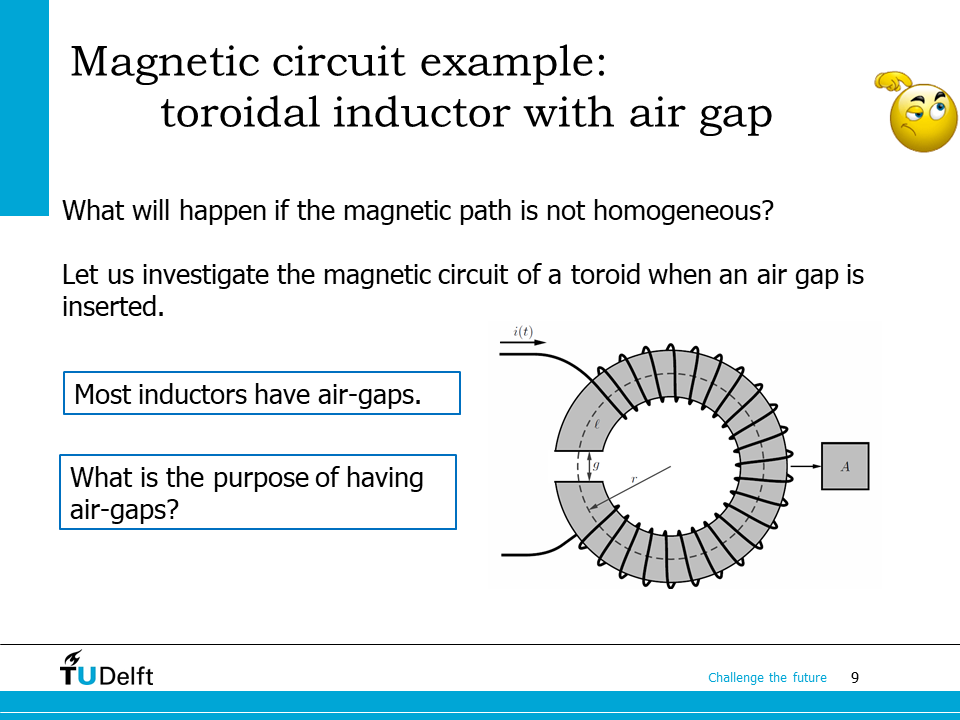
Most inductors have air gaps inserted to the magnetic core. The purpose of having air gaps is to extend the operation range: the air gap can prevent the magnetic core from saturation at large current. As we will see later in this lecture.
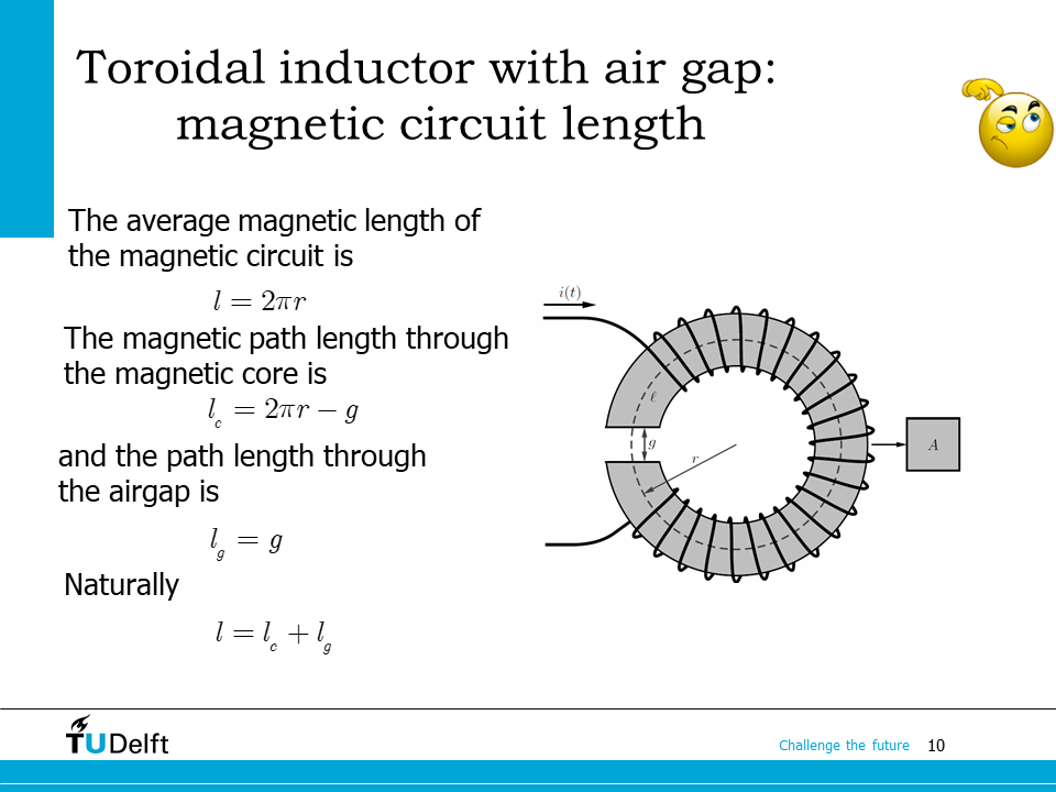
The air gap length is \(g\), while the radius of the core is \(r\). The magnetic path in the core will have a length of \(l_c = 2\pi r - g\), while the path in the air has a length of \(l_g = g\).
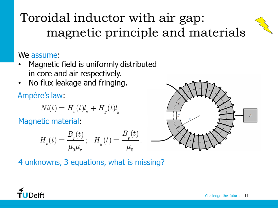
Before doing the calculation by applying the two laws, we have to make some assumptions as follows:
The magnetic flux density is uniformly distributed in the cross section of the core and the air gap;
There is no leakage, i.e., all the magnetic flux leaving the core will penetrate through the air gap and enter the other side of the core;
There is no fringing effect, i.e., all the magnetic flux does not exceed the edges of the air gaps.
The leakage and fringing effect will be demonstrated later in the coming slide.
Based on the assumptions above, by applying the Ampere’s law and the material properties, we will have the 3 equations listed on the slide.
However, There are 4 unknowns: the magnetic field strength in the core and the air \(H_c\) and \(H_g\), the magnetic flux density in the core and the air \(B_c\) and \(B_g\).
In order to solve the 4 unknowns, we have to find a 4th equivalence.
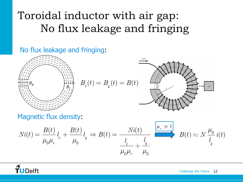
Here is where the assumptions play a role. Because we assume there is no leakage and fringing effect, the flux lines in the core and the air gap will be continuously and uniformly distributed as shown on the left. So the flux density in the core and the air gap will be the same \(B_g(t) = B_c(t) = B(t)\). Based on this and the 3 equations on the previous slide, we have
Then the flux density is solved as
Since the permeability of the ferromagnetic core is far larger than that of the air gap \(\mu_r \gg 1\), the \(\frac{l_c}{\mu_r\mu_0}\) would be negligible. Therefore the flux density will be dominate by the air gap part
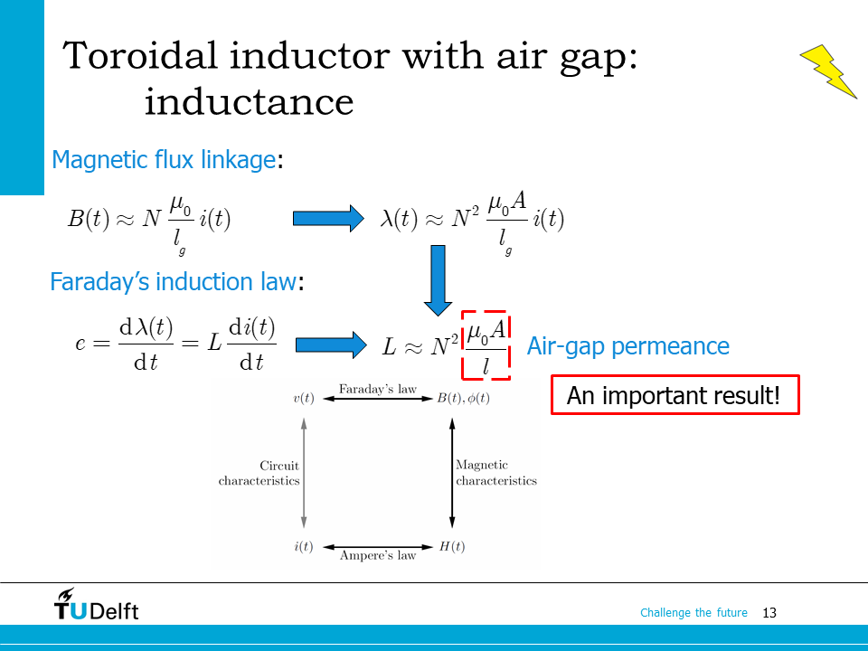
By solving magnetic flux linkage from flux density again, we can see the inductance is dominated by the air gap part as well:
Here will can see \(L = N^2\mathcal{P}\) still holds.
The above problem can also be solved by applying the magnetic circuit concept, as shown below:
The magnetic reluctance of the complete magnetic circuit is
The magnetic flux flows through the core is the same as that through the air based on the above assumptions, so we have
The flux density and the flux linkage are
which are the same as those derived by applying Ampere’s law directly. Note that the total permeance is
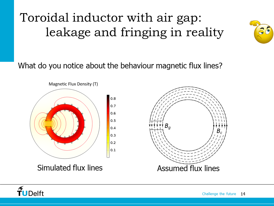
Be aware that the previous calculations are based on the assumptions: \(B\) is uniformly distributed, and there is neither leakage nor fringing effect. Therefore the calculation is just an approximation with sufficient accuracy.
On this slide, a more accurate flux line distribution simulated from finite element method is compared with the assume one. It can be see that in practice, not all magnetic flux go through the air gap. The flux bypassing the air gap is called leakage flux.
Not all flux penetrating the air gap right under the cross section. This phenomenon is called fringing effect. In engineering, we usually account for the fringing effect by using a larger air gap cross sectional area in calculation. But this is outside of the scope of the course.
15.3. Coupled coils#
Having studied one individual inductor from the magnetic field point of view, let us move on to the case where two coils are coupled together through the same magnetic core, which has been discussed briefly in Flyback Converter part of the course. This time we will analyze it in detail.
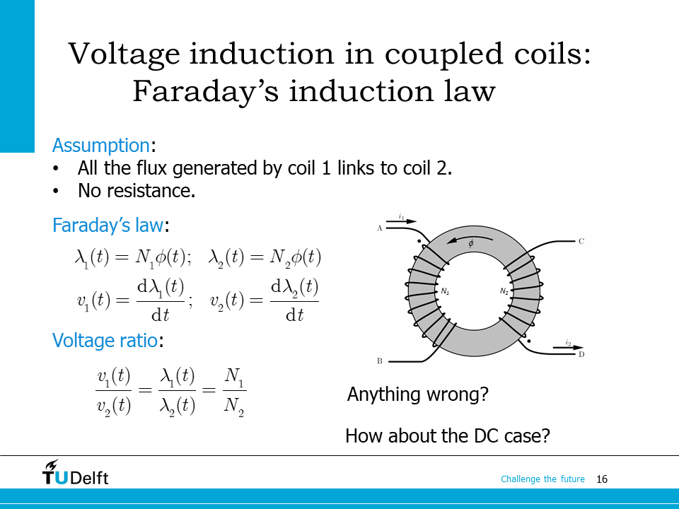
As we can see here, coil 1 and 2 are wounded on the same toroidal core. To simplify our analysis, we first assume the two coils are fully coupled, i.e., all magnetic flux links coil 1 also links coil 2, and there is no resistance in the two coils.
Based on the assumptions above, we know the flux linkages of the two coils would be \(\lambda_1(t) = N_1\phi(t)\) and \(\lambda_2(t) = N_2\phi(t)\) respectively, since they share the same flux. From Faraday’s law, we know the induced voltage ratio is exactly the flux linkage ratio. Because there is no resistance, the induced voltage and the terminal voltage would be the same (Kirchhoff’s law), so
Attention
The equation above is only valid for AC voltages. If DC voltage is applied, the induced voltage in both coils will be zero.
15.4. Ideal transformer#
As we have learnt in the linear circuit courses, two coupled coils form a transformer. Let us start analysing the transformer with ideal assumptions.
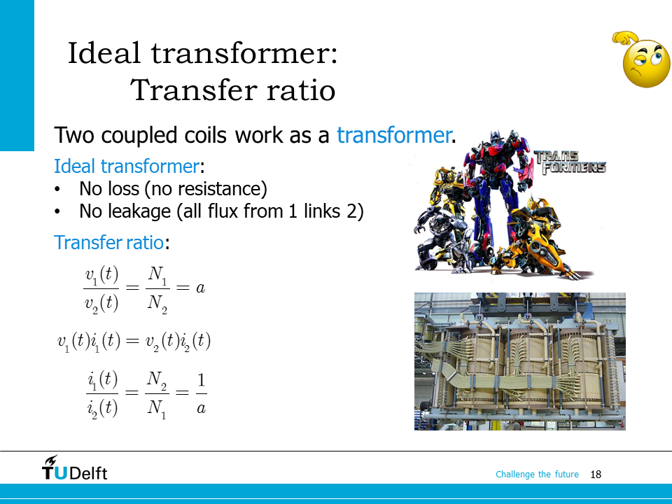
Because of the two ideal assumptions (no resistance, no leakage), the two coupled coils exhibit a lossless, fully coupled behaviour. Therefore, they can be treated as an ideal transformer.
The voltage transfer ratio will be the turns ratio \(a = N_1/N_2\). Because of the lossless assumption, all power from the primary side will transfer to the secondary side or vice versa, so the current transfer ratio is the inverse of the voltage transfer ratio \(i_1/i_2 = 1/a = N_2/N_1\).
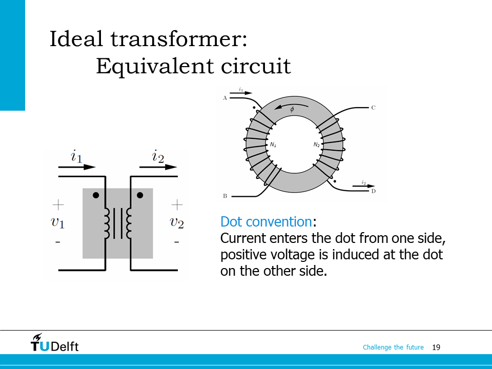
We use dot convention to represent the polarities of the two coils in circuit schematics of coupled coils. We gave the defition of it in Flyback Converter and here we repeat it.
Dot convention
When the reference direction of a current enters the dotted terminal of a coil, the reference polarity of the voltage that it induces on the other coil is positive at the dotted terminal. We can also state it differently. When the current enters a coil at the dotted terminal then the current flow due to the induced voltage on the other coil will leave the coil at its dotted terminal.
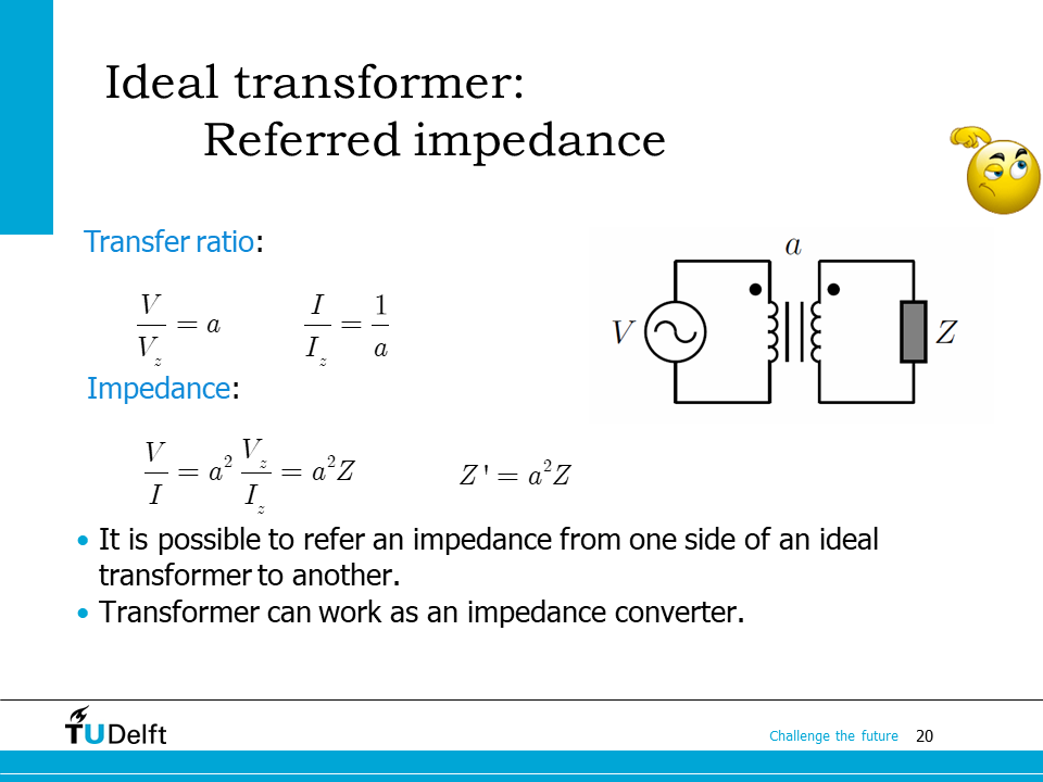
From the voltage transfer ratio \(a\) and the current transfer ratio \(1/a\), we can see if there is a load impedance on the secondary side \(Z\), it will be equivalent to having an impedance of \(a^2Z\) on the primary side, or if there is an impedance of \(Z^\prime\) on the primary side, it would be equivalent to an impedance of \(Z^\prime/a^2\) on the secondary side.
So it would be possible to refer the impedance from one side to another by applying the impedance transfer ratio. In such way, a transformer can work as an impedance converter.
15.5. Homework#
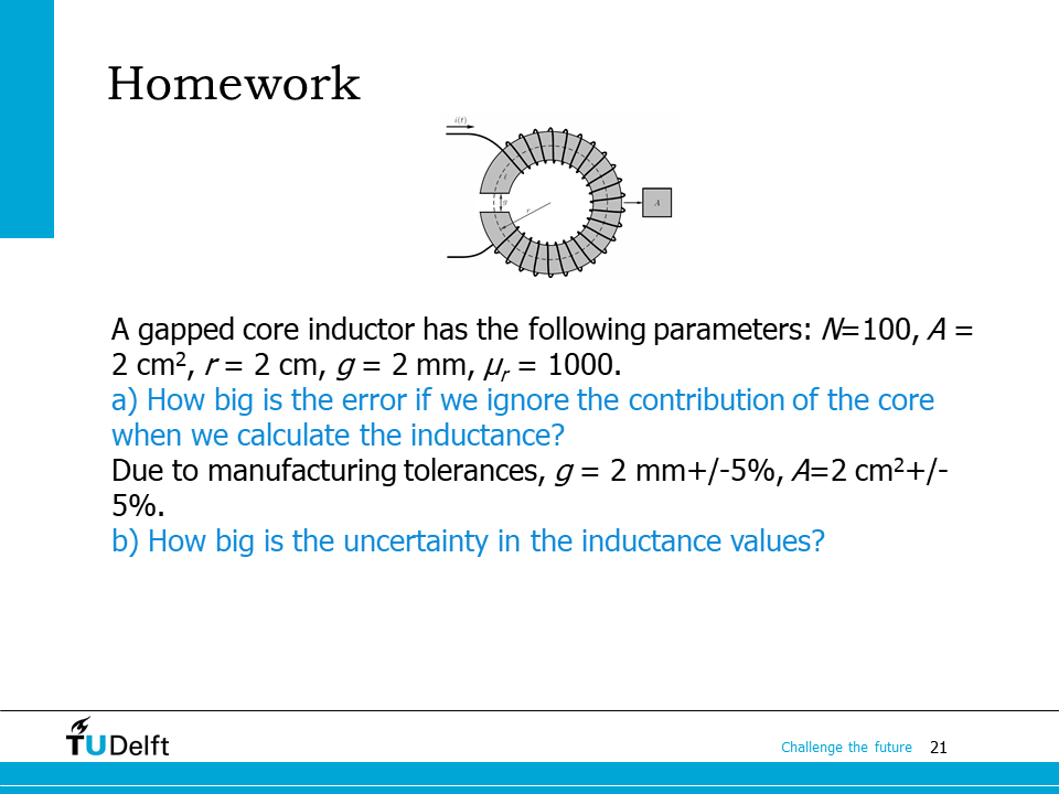
Let’s use this homework to practice what we have studied in this lecture. Please first try to solve it yourself and check the block and the code below for the right answer.
Click here for solution
Show code cell source
import numpy as np
N = 100.0
A = 2.0e-4 # convert to m^2
r = 2.0e-2 # convert to m
g = 2.0e-3 # convert to m
mur = 1000
mu0 = 4*np.pi*1.0e-10 # permeability of air
g_min = g*0.95
g_max = g*1.05 #+/- 5% tolerance
A_min = A*0.95
A_max = A*1.05
lc = 2*np.pi*r - g
# a. influence of air gap
# if we do not neglect the core
# magnetic permeance is:
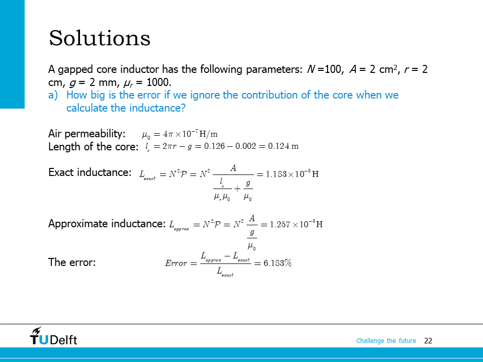
P_with_core = 1/(lc/mu0/mur/A + g/mu0/A)
# inductance is
L_with_core = N**2*P_with_core
# if we neglect the core
# magnetic permeance is
P_without_core = mu0*A/g
L_without_core = N**2*P_without_core
print(f'a. The error introduced by neglecting the core is {((L_without_core - L_with_core)/L_with_core):.3%}.')
# b. uncertainty in inductance
# max inductance -> smallest g, largest A
# min inductance -> largest g, smallest A
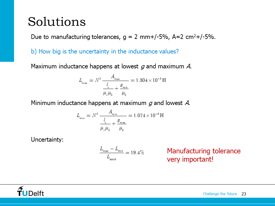
L_max = N**2/((2*np.pi*r-g_min)/mu0/mur/A_max + g_min/mu0/A_max)
L_min = N**2/((2*np.pi*r-g_max)/mu0/mur/A_min + g_max/mu0/A_min)
print(f'b. The uncertainty because of the manufacturing tolerance of the core is {((L_max - L_min)/L_with_core):.3%}.')
a. The error introduced by neglecting the core is 6.183%.
b. The uncertainty because of the manufacturing tolerance of the core is 19.451%.
As we can see from the calculation above, the error introduced by the manufacturing tolerance is much larger than that introduced by neglecting the contribution from the core. It tells us the conclusions shown on the slide.
Because of the air gap, the inductor is also less prone to saturation, because the inductance is less sensitive to the permeability change of the ferromagnetic material. So most inductors have an air gap to make the inductance value more stable.
In transformers, an air gap is usually not needed because the primary side current and the secondary current will create opposite magnetic field under normal operation. The magnetising current is actually corresponding to the \(Ni\) difference between them. There is no saturation as long as the voltage does not exceed the rated value, and an air gap in transformer does not prevent the saturation if the input voltage is too high.
An exemption is the “transformer” or coupled coils in certain power electronics topologies, air gaps are introduced either to tune the inductance to trigger resonance, or to prevent saturation so that it stores more energy for conversion. For example, in a flyback converter, the “flyback transformer” is actually an inductor with a secondary coil. When the switch is on, secondary current is 0, while the primary current magnetises the core; when the switch is off, primary current is turned off, and the secondary current magnetises the core. The magnetising current is directly the input current or the output current, which can be very large, so we need an air gap in the core to prevent saturation.