14. Magnetic circuit Principles#
14.1. Introduction#
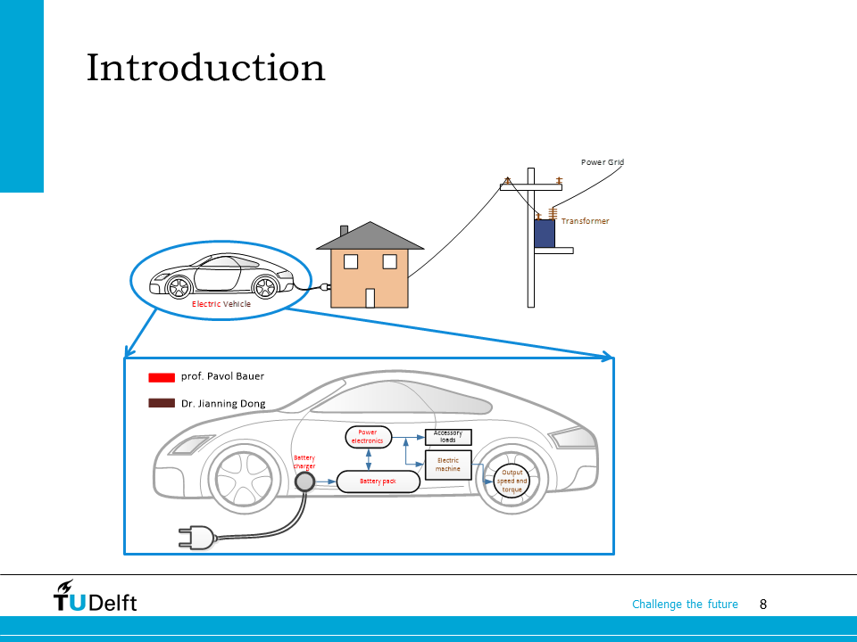
In this module, we will study the basic magnetic principles to lay the foundation for analysis of magnetic components in electrical energy conversion, including inductors, transformers and electrical machines. As we can see here, the brown letters indicate where magnetics plays a role in electrical energy conversion.
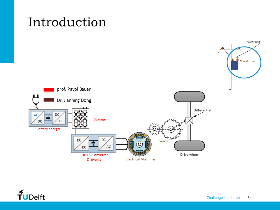
This slide shows in more detail. Fro this lecture on, we will move from power electronics, to the world of electromechanics, where magnetics principles and electromechanical energy conversion are used to convert energy between the electrical world and the mechanical world.
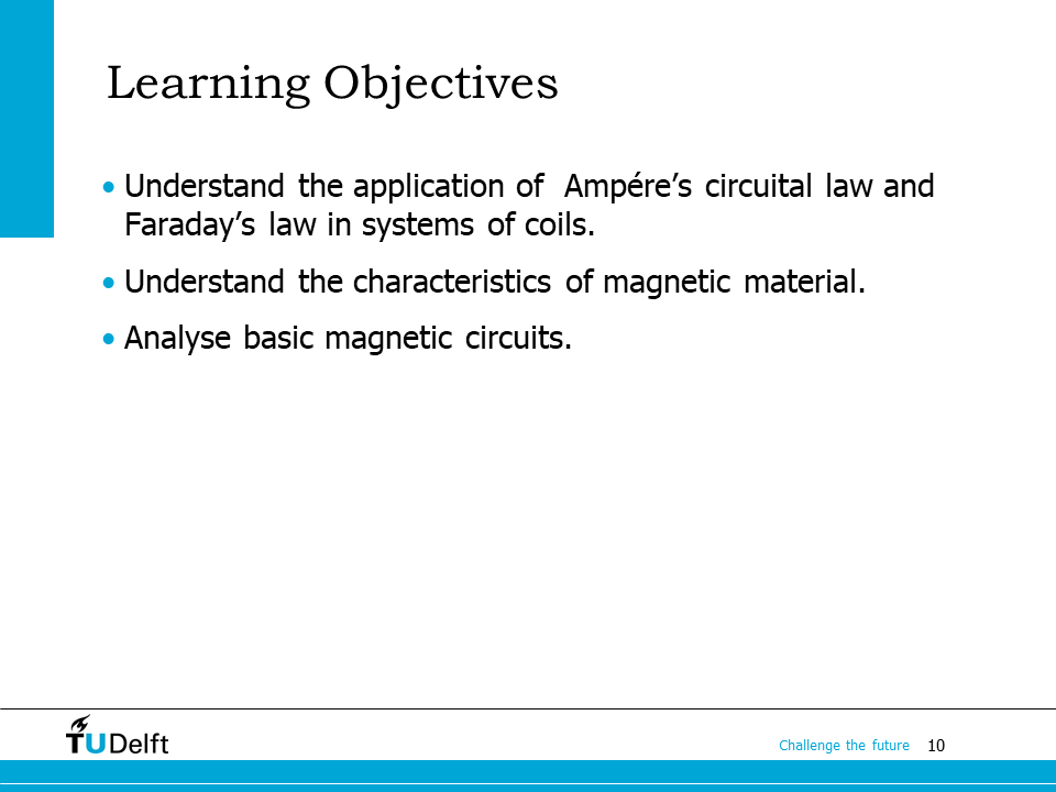
Learning objectives are listed on the slide. We will start with reviewing of the two basic magnetic laws. Then review the magnetic properties of different materials. In the end, we will study the basic magnetic circuits and us it to solve the inductance of an inductor.
14.2. Revisit magnetic principles#
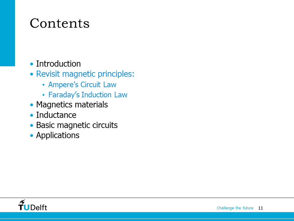
The contents of the lecture are shown here.
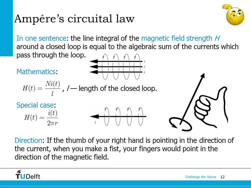
French physicist Andre-Marie Ampére found that the electric current creates the magnetic field. The relationship is descibed as Ampére’s circuital law. The statement of the law is written in one sentence: the line integral of the magnetic field strength \(H\) around a closed loop is equal to the algebraic sum of the currents which pass through the loop.
Here the magnetic field strength \(H\), also called magnetic intensity or magnetic field intensity, represents the part of the magnetic field in a material that arises from an external current.
The slides shows a simple case, where a very long and thin wire carrying a current \(i(t)\) in the vacuum, the magnetic field strength at a distance \(r\) from the wire will be as shown on the right of the slide. The directions of the current and the magnetic field are related to each other via the right hand rule. The magnitude of the magnetic field strength is in this case
Note
The magnetic field strength is a vector. The equation above just shows its magnitude. The direction is determined by the right hand rule, in such case, as indicated by the grey arrows.
In general, if \(N\) turns of wires all carrying a current \(i(t)\) is enclosed, and the magnetic field strength is uniformly distributed along the closed loop to apply Ampére’s law, we have
where \(l\) is the length of the closed loop.
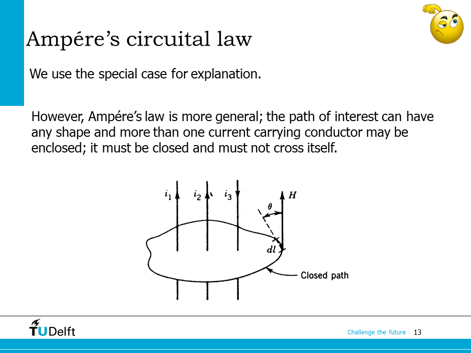
In the previous slide, we use the special case for explanation, however, in practice, Ampére’s law is more general; the path of interest can have any shape and more than one current carrying conductor may be enclosed; it must be closed and must not cross itself. A more general mathematical statement of Ampére’s law is
where \(\mathbf{H}\) is the magnetic field strength vector, \(C\) is the closed loop to apply the integral, \(\mathrm{d} \mathbf{l}\) is the differential of the loop \(C\), and the right hand side of the equation represents the total current enclosed by the loop \(C\).
The unit of the magnetic field strength is \([\mathrm{A/m}]\),
In 1831 the English chemist and physicist Michael Faraday observed that when two coils are placed next to one another a current is induced in the second coil whenever the current in the first is switched either on or off.
Incidentally across the Atlantic in Albany, New York, Joseph Henry made the same discovery at roughly the same time. However, Faraday was first to publish his results and the law describing this phenomena bears his name today. Henry’s name is used as the unit of inductance since it is a consequence of the Faraday’s Induction Law.
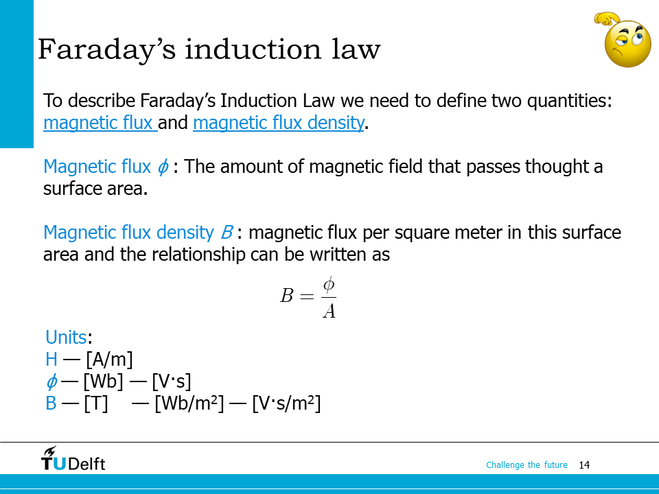
To describe Faraday’s Induction Law we need to define two quantities: magnetic flux \(\phi\) and magnetic flux density \(B\). Magnetic flux is a term used to describe the amount of magnetic field in a given region. Magnetic flux is denoted by \(\phi\) and is measured in Weber, \([\mathrm{Wb}]\), named after Wilhelm Eduard Weber, a German physicist who first devised a system of absolute measurements for electric currents. We will see later that \([\mathrm{Wb}]\) is equivalent to \([\mathrm{V\cdot s}]\).
Magnetic flux density is defined as the magnetic flux per square meter in a specific unit surface area and the relationship can be written as
if we assume \(B\) is perpendicular to the surface area \(A\), and is uniformly distributed.
For general case, we have to describe the relationship between magnetic flux density and magnetic flux in vectors:
where \(\mathbf{S}\) is the area vector of the surface, \(\mathbf{B}\) is the magnetic flux density vector.
\(B\) is measured in Tesla or \([\mathrm{T}]\), which is named after the brilliant Croatian-American inventor and engineer Nikola Tesla, and is also equivalent to \([\mathrm{Wb/m^2}]\), \([\mathrm{V\cdot s/m^2}]\) or \([\mathrm{N/A/m}]\).

The magnetic flux and magnetic flux density are invisible, but in modern engineering, we often use software based numerical simulation (mostly finite element method), to solve them and visualise them.
Here it shows two examples, which are obtained from finite element simulation of an E-core inductor (top) and a permanent magnet synchronous machine (bottom). Only a sectional cut of them is simulated. The flow of magnetic flux is represented as lines in the two figures. The magnetic flux density distribution is represented as colors, as shown in the legends attached to the figures. It can be seen that the denser the magnetic flux lines, the higher the flux density.
What can you observe from the two figures?
Most of the flux lines go through a main path shaped by the magnetic core;
There are leakages flux lines which do not go through the air gap;
There are flux lines which go through the air gap, but goes out of the edges of the magnetic core;
It can also be seen from the bottom figure, there are 6 magnetic poles.
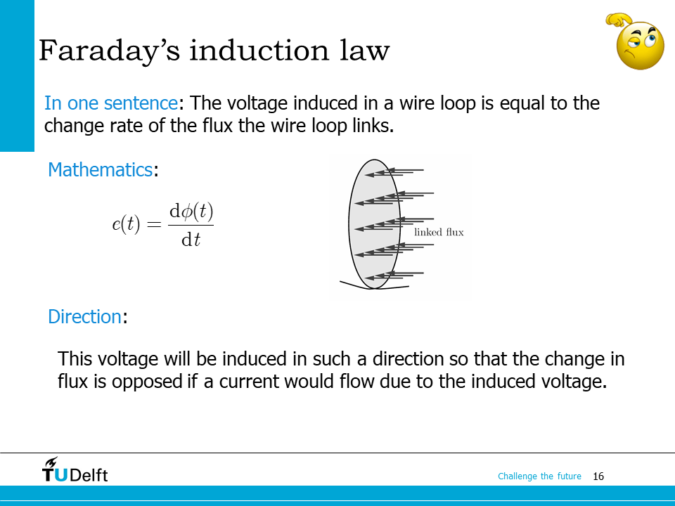
Faraday’s induction law states that any change in the flux “contained” by a wire loop will induce a voltage in the wire. This voltage will be induced in such a direction so that the change in flux is opposed.
In basic terms the law states that the magnitude of the induced voltage is
where \(\phi(t)\) is the magnetic flux going throw the surface area enclosed by the wire loop, or alternately the flux linked by the loop. The direction of \(e(t)\) is that the current caused by it will oppose the change in the original flux.
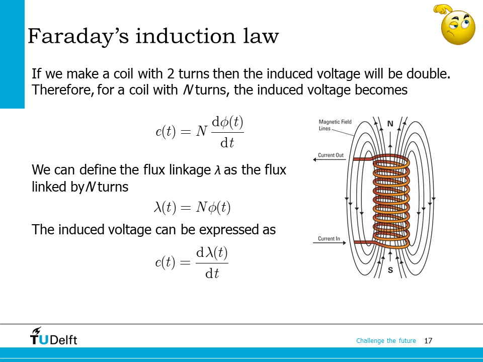
In practice, we often make a coil with multiple number of turns to add up the induced voltage. For \(N\) number of turns wounded in the same loop, the total induced voltage is
Here we can define \(N\phi(t)\) as the flux linkage of the coil, which is denoted by \(\lambda\), so we have
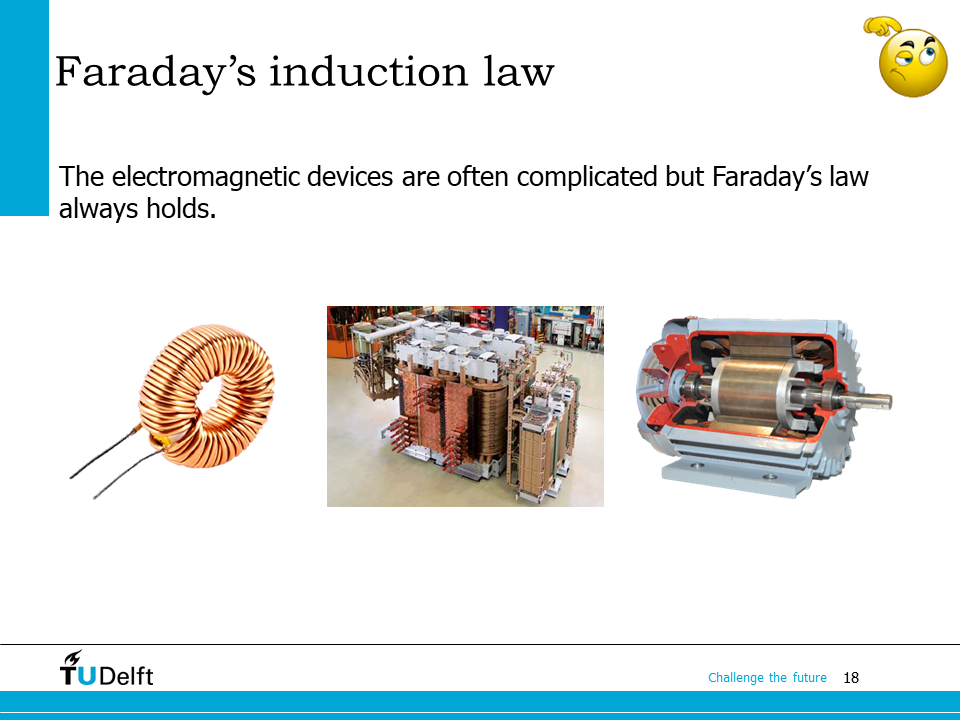
All electromagnetic devices, including inductors, transformers and electrical machines operate based on the two laws we reviewed. No matter how complicated the devices are, we are always able to analyse them using the two laws.
14.3. Magnetic materials#
From Ampére’s law, we know how magnetic field strength \(H\) is related to the current \(i\). From Faraday’s law and the definition of flux linkage, we know how the magnetic flux density \(B\) is related to the induced voltage. To fully link the electrical quantities with the magnetic quantities, we still have to know how \(H\) is related to \(B\), which is determined by the magnetic characteristic of materials.
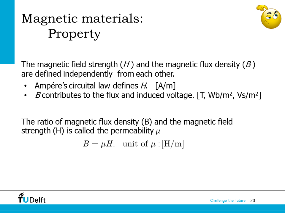
How well a material is magnetised (indicated by magnetic flux density \(B\)) by certain strength of magnetic field (indicated by \(H\)) is described by its magnetic characteristic.
For linear magnetic material, \(B\) is linearly proportional to \(H\). The ratio between them is called the permeability \(\mu\).
The unit of \(\mu\) is [\(\mathrm{H/m}\)], where \([\mathrm{H}]\) is the unit of the inductance. We we see later how \(\mu\) is linked to inductance.
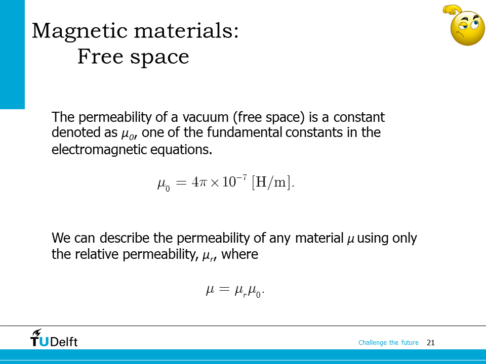
The permeability of the vacuum (free space) is a constant, which is
It is handy to refer the permeability of certain material to \(\mu_0\),
where \(\mu_r\) is called the relative permeability.
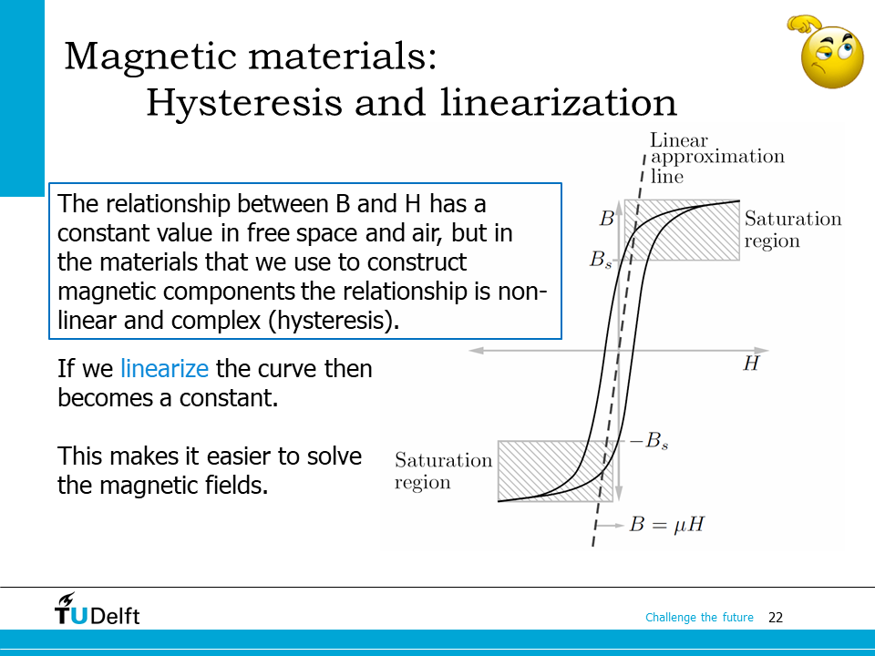
The permeability in free space and air is constant, and we are able to treat them as linear magnetic material. However, in most of the electromagnetic devices, we have to deal with nonlinear magnetic materials, for example the magnetic core made of silicon steel, or ferrites.
A typical relationship between the magnetic field strength and the magnetic flux density in the nonlinear magnetic material is shown on the slide. Here we can observe that
The relationship between H and B is not linear
The forward and return paths are not the same, the relationship clearly exhibits a form of hysteresis.
When the magnitude of the flux density \(B\) is high, the ratio between \(B\) and \(H\) gets smaller, i.e., \(\mu_r\) decreases, which is called saturation.
Hysteresis
The definition of hysteresis is a process whose output not only depends on the value of the input, but also on the historical input.
It takes energy when the hysteresis magnetic material is magnetised and demagnetised in a cycle, which is in proportion to the area enclosed by the hysteresis loop, and is called hysteresis loss.
It is possible to describe the hysteresis behaviour using advanced mathematical tools, however, in practice when the flux density \(B\) is lower than the saturation value \(B_s\), it is often accurate enough to approximate it by applying the assumptions below:
We will ignore the hysteresis nature of the relationship. We therefore assume that the forwards and backwards paths are the same, which is the centre line of the original hysteresis loops.
Since \(B<B_s\), we assume the magnetic property is linear, i.e., we can use \(B=\mu H\) to approximate the relationship between \(B\) and \(H\).
Therefore, we are able to use an average line, shown as the “linear approximation line” in the figure, to approximate the magnetic characteristics of an nonlinear magnetic material when it is not saturated.
In practice, we often design the electromagnetic devices so that it operates at the corner point of saturation to reduce the size, therefore it is critical to consider the nonlinear behaviour. In that case, we can use more advanced mathematical tools, such as finite element method to solve the magnetic field. But this is outside of the scope of this course.
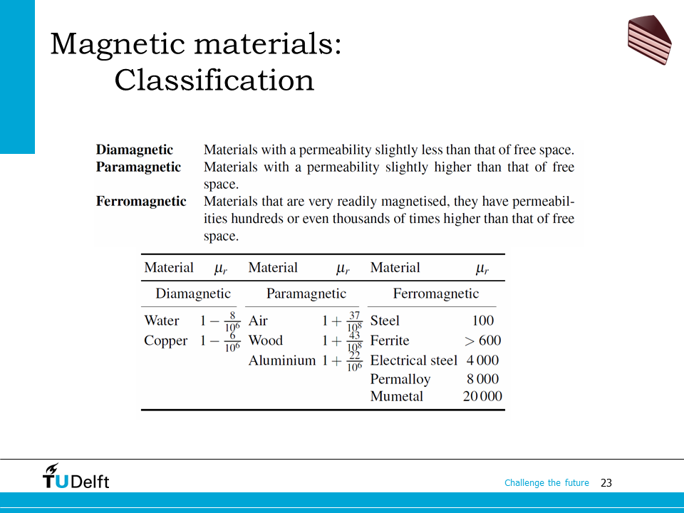
We can categorise the magnetic characteristics of the materials we are likely to encounter in electrical energy conversion systems into three broad categories:
- Diamagnetic
Materials with a permeability slightly less than that of free space.
- Paramagnetic
Materials with a permeability slightly higher than that of free space.
- Ferromagnetic
Materials that are very readily magnetised, they have permeabilities hundreds or even thousands of times higher than that of free space.
The relative permeabilities of some typical materials are listed on the slide. It can be seen that for diamagnetic and paramagnetic materials, we can assume that \(\mu_r=1\).
Ferromagnetic materials have much higher relative permeability, which make them ideal medias to guide the magnetic flux. Therefore, they are often used as magnetic cores in inductors, transformers or electric machines
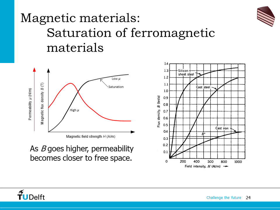
Here let us check the saturation behaviour of the ferromagnetic materials. On the left hand side, it shows a typical \(B-H\) curve* and a \(\mu-H\) curve of a ferromganetic material, which is approximated from the average of the hysteresis loop. As we can seen, if \(B\) surpasses \(B_s\), as \(B\) goes higher \(\mu\) gets closer to \(\mu_0\). From the right hand side, we can see, if cast iron or steel are used, we will have lower saturation flux density \(B_s\) and narrower linear range. Therefore, in electrical engineering, silicon is often added to steel to improve its magnetic performance, which is called electrical steel or silicon steel.
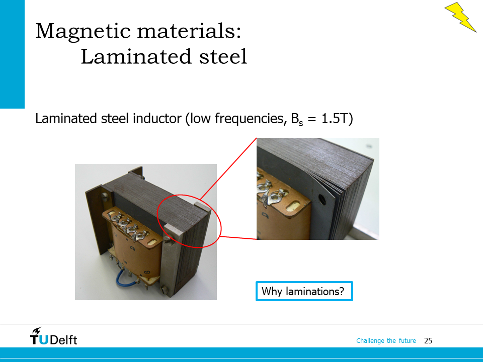
Among various ferromganetic materials suitable for making magnetic core, silicon steel is often used for low frequency application. Since steel is conductive, there will be eddy current flow inside the core when AC magnetic field is applied (voltage is induced inside the core according to Faraday’s law, which gives rise to current circulating inside the core). To limit the loss caused by the eddy current, silicon steel should be laminated to increase the resistivity of the core when it is used in AC applications. The eddy current loss is also the reason why the application of silicon steel is limited to low frequency applications.
The saturation flux density of the silicon steel is often around \(\mathrm{1.5~T}\).
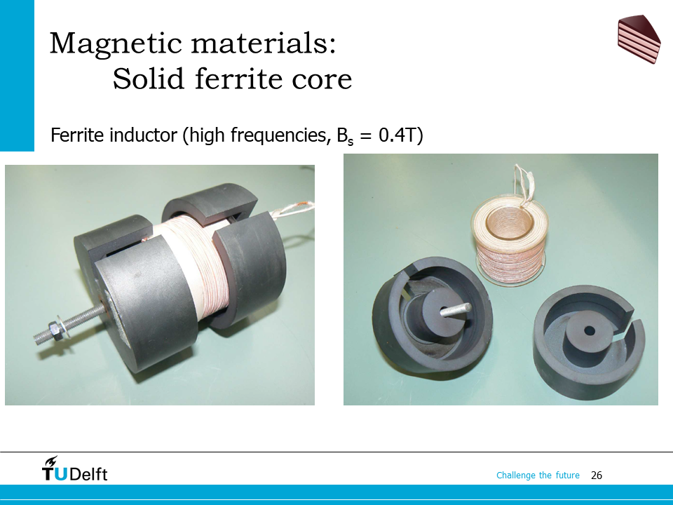
For high frequency applications, ferrite core is often used. The ferrites used for magnetic core are also called soft ferrites, since they have very small hysteresis loop, therefore, are easier to be magnetised and demagnetised without dissipating much energy (hysteresis loss). These materials have high resistivity, which prevents eddy currents in the core, and hence it is possible to use solid ferrite cores without laminating.
The saturation flux density of the ferrites is usually around \(\mathrm{0.4~T}\), which is much lower than that of silicon steel, however, their lower loss make them an ideal choice for high frequency applications.
14.4. Inductances#

We are able to link the electrical quantities with the magnetic field quantities using the two magnetic laws. However \(B\) and \(H\) are field quantities, which are not intuitive to solve. Hereby we introduce the circuit component: inductance, to better link the two worlds.
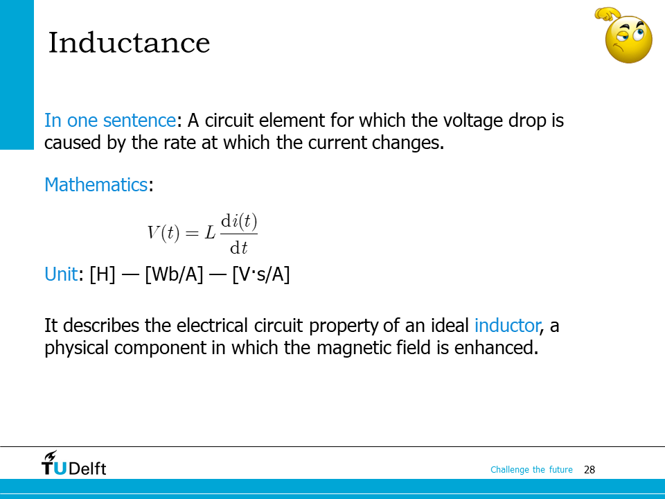
In one sentence, we can define the inductance as a circuit element for which the voltage drop is caused by the rate at which the current changes, or mathematically, as
The unit of the inductance \(L\) is \([H]\), which is equivalent to \([\mathrm{Wb/A}]\) or \([V\cdot s /A]\). It describes the electrical circuit property of an ideal inductor, a physical component in which the magnetic field is enhanced.
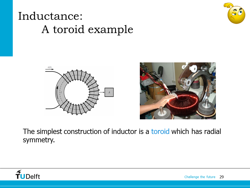
Let’s use a toroidal core inductor as shown on the slide to show how inductance is used to link electrical circuits with magnetics.
The right hand side shows how a toroidal core inductor is wounded in practice.
14.5. Basic magnetic circuits#
We will introduce the concept of magnetic circuit to analyse this inductor. A magnetic circuit is made up of one or more closed loop paths containing a magnetic flux. So magnetic flux to a magnetic circuit is like current to an electrical circuit. Accordingly, the magnetic excitation \(Ni\) in Ampere’s law (source of magnetic flux) is magnetomotive force (MMF), and is like voltage in an electrical circuit. The magnetic reluctance \(\mathcal{R}\) is defined as the ratio between MMF and magnetic flux of a certain segment of the magnetic circuit, and acts like the resistance in an electrical circuit.
\(\mathcal{R}\) can be calculated from the cross sectional area of the magnetic circuit path \(A\), the permeability of the material, and the length of the magnetic circuit \(l\):
Accordingly, permeance \(\mathcal{P}\) is defined as the inverse of the reluctance, which is like conductance to resistance in an electrical circuit.
Based on the fundamentals given above, let’s analyse the toroidal core inductor using the magnetic circuit approach.
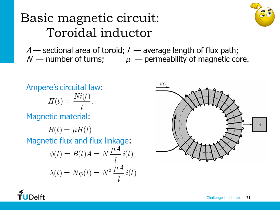
First the magnetic circuit is the closed loop formed by the magnetic core, since the magnetic flux is bounded by it.
If we apply Ampere’s circuital law and consider the magnetic characteristic of the core, we are able to derive the equations shown on the slide. Alternatively, we can use the magnetic circuit approach as follows.
The MMF in the magnetic circuit is
The reluctance of the magnetic circuit is
Finally, the magnetic flux is calculated
The flux linkage linked by the coil is calculated by \(\phi\) multiplying \(N\)
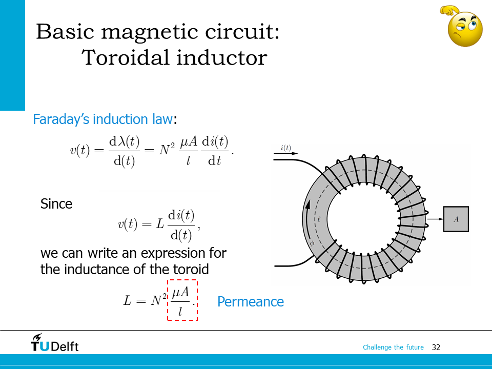
Then if we apply Faraday’s law to the flux linkage, the induced voltage is obtained as shown on the slide. By comparing the equation to the mathematical description of the inductance in the electrical circuit, we can see the inductance \(L\) is actually
Apparently, \(L\) is proportional to the permeance of the magnetic circuit:
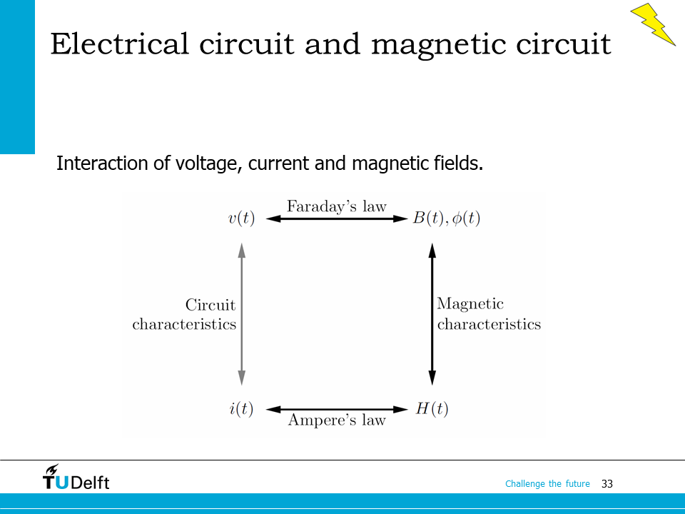
Now we are able to complete the loop to couple the magnetic circuit with the electrical circuit. With the tools developed in the previous slides we can now attack quite a few magnetic circuit problems with confidence.
The interactions of the current, magnetic field and the voltage is visualised on the slide. We will use these steps and the theory developed to discuss a few circuits in the coming lectures.
14.6. Applications#
In the end of the lecture, let’s check some applciation examples of inductors.

Here it shows the current limiting power reactor (a giant inductor) in a power substation, it is used to limit the short-circuit current in the power grid when fault occurs. Usually an air core is used instead of ferromagnetic material core in such application to avoid saturation caused by high short circuit current.
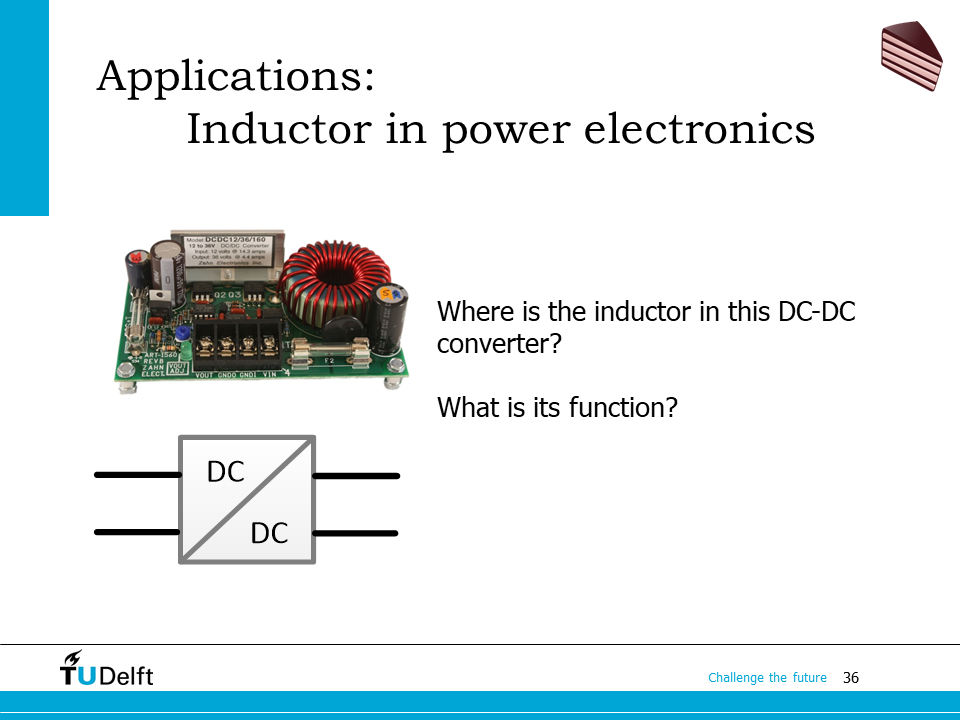
In the previous module, we have learnt that the inductor is used in various DC-DC converters, which is used to store energy when the switch is turned on then release it when the switch is off, so that we are able to change the voltage level from one to another without significant loss.