DC Drive

21. DC Drive#

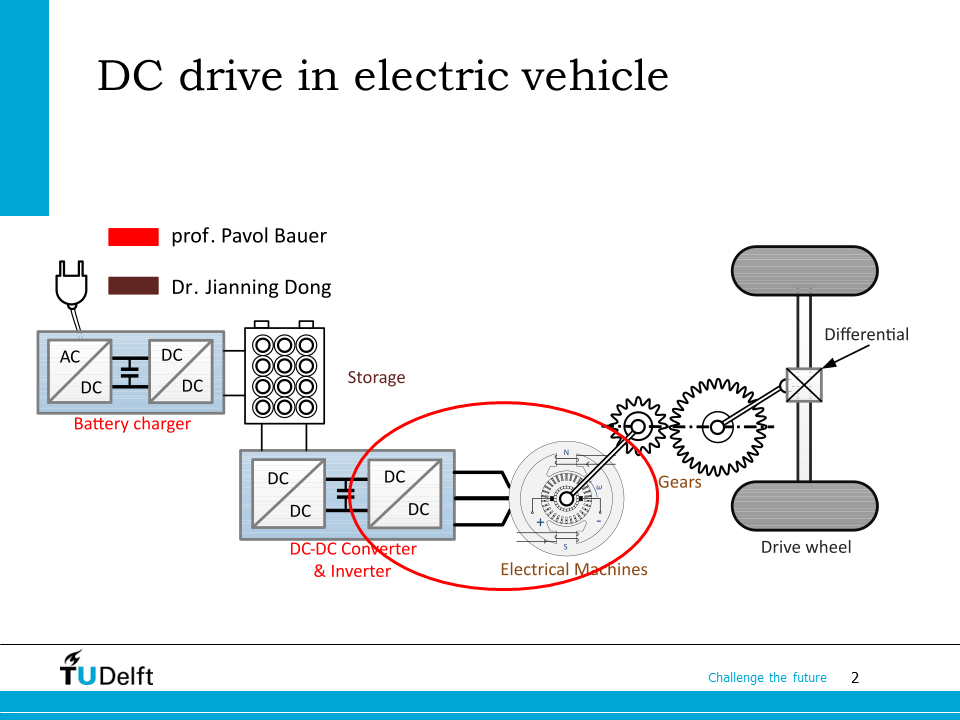
In this lecture, the DC drive will be studied. A DC drive system composes of the DC/DC converter and a DC machine, as is shown on the slide.

Note

In practice, the DC drive system is rarely used for propulsion of electric vehicles, mainly because the brush-commutator mechanism has reliability issues because of wearing and the power density of it is inferior to AC drive systems.

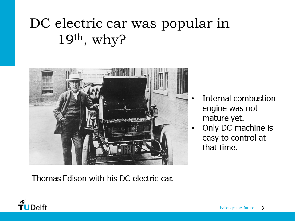
Although the DC drive is not extensively used in electric vehicles nowadays, because of the reasons mentioned above. However, in the 19th century, the first engine powered cars were most powered by DC motors. The reason was the internal combustion engine (ICE) technology was not mature enough for mass production yet, and the power electronics converters were not invented yet. The speed of the DC machine can be regulated by adding variable resistor into the armature or the field circuit, which made it suitable for car application at that time.

Since 1960s, the invention of power semiconductors provide the possibility to control the DC motor more efficiently without extra losses caused by external resistors. In this lecture, we will study how to use modern DC-DC converters to make a DC drive system, and how to regulate the converter for speed control.

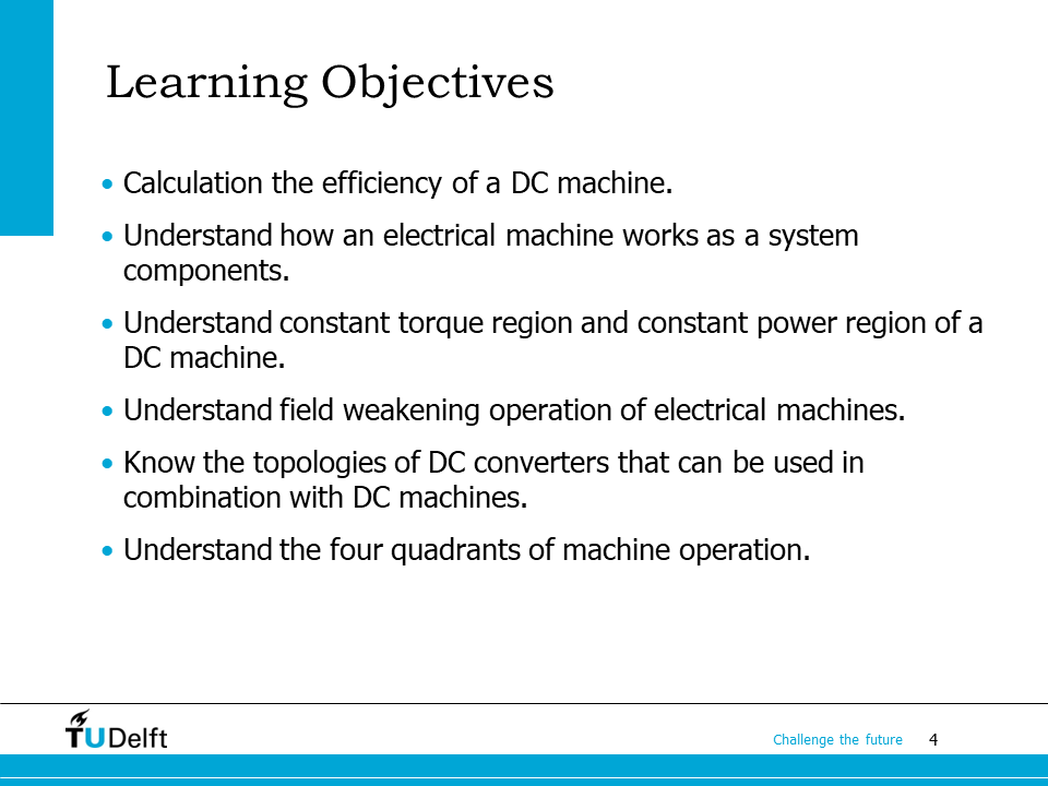
After taking this lecture, we should be able to meet the objectives listed on the slide. Particularly, we need to understand the concept of constant torque and constant power operations, and tell how field weakening works. The DC-DC converter topologies suitable for various operation modes (1-quadrant, 2-quadrant, 4-quadrant) will also be studied.

21.1. DC machine efficiency#

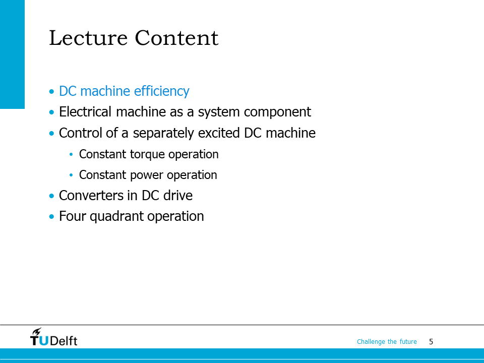
We first study the efficiency calculation of the DC machine.

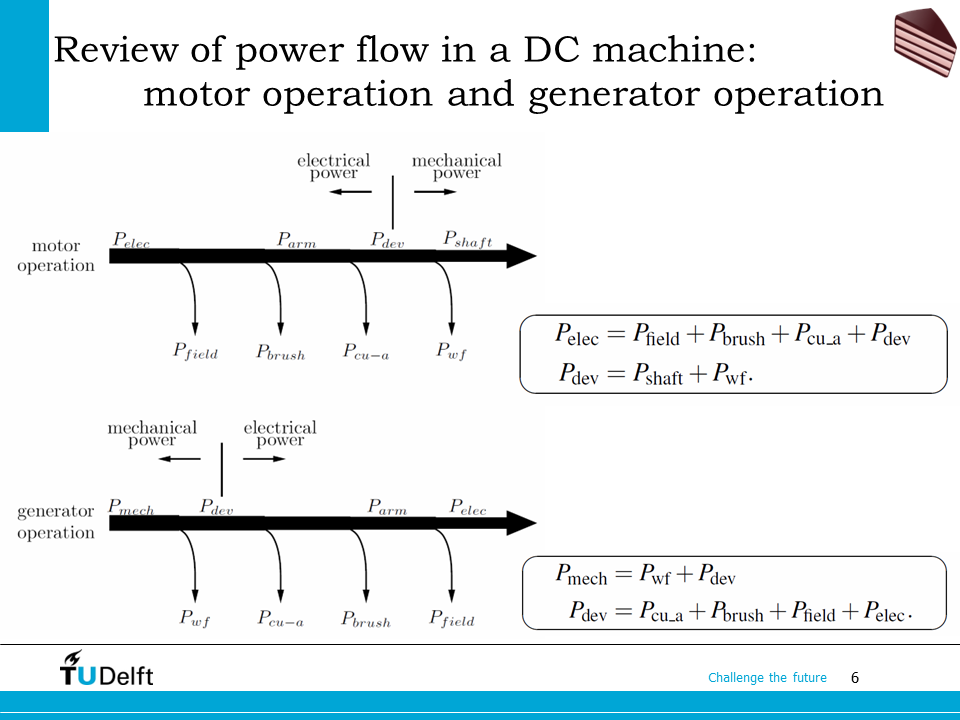
As we have learnt in the last lecture, the power flow in the DC machine changes direction as the operation modes change from motor operation to generator operation.

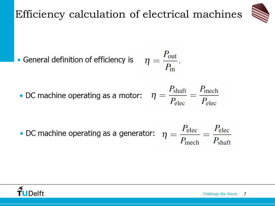
For general electrical machines, the efficiency is defined as the ratio between the output power and the input power.

In the motor operation mode, the output power is the mechanical power delivered to the shaft, i.e.,

\[ \eta = \frac{P_{shaft}}{P_{elec}} = \frac{P_{mech}}{P_{elec}}. \]

In the generator mode, the output power is the electrical power delivered to the electrical terminal, while the input power is the mechanical power applied on the shaft, i.e.,

\[ \eta = \frac{P_{elec}}{P_{shaft}} = \frac{P_{elec}}{P_{mech}}. \]

Attention

Pay attention to operation modes and power flow directions when calculating input power, output power and efficiencies of all electrical machines. This is important in the practical module 2 as well.

21.2. Electrical machine as a system component#

The electrical machine does not operate alone. It has to serve for a larger system in practice.

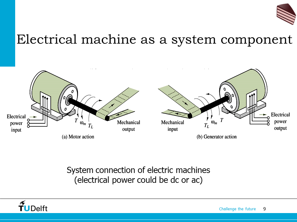
The electrical machine operates as an electromechanical energy conversion component in larger systems.

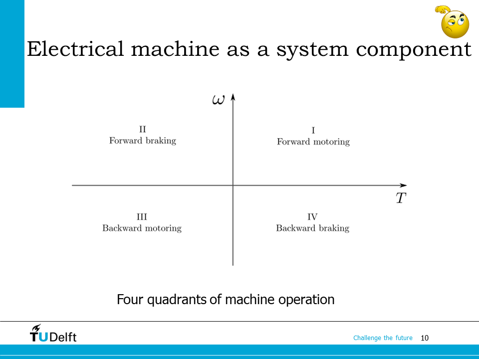
Similar to the classification of DC-DC converters, depending on the rotating direction and the power flow direction, we can classify the operation of the electrical machine in a system into four quadrant. If we put the angular speed \(\omega\) on the y-coordinate, and the torque \(T\) on the x-coordinate, the operation point of an electrical machine can be located in one of the 4-quadrants:

I: forward motoring, \(\omega>0\) or \(e_a > 0\), and \(i_a > 0\);
II: forward braking, \(\omega>0\) or \(e_a > 0\), and \(i_a < 0\);
III: backward braking, \(\omega < 0\) or \(e_a < 0\), and \(i_a > 0\);
IV: backward motoring, \(\omega < 0\) or \(e_a < 0\), and \(i_a < 0\);

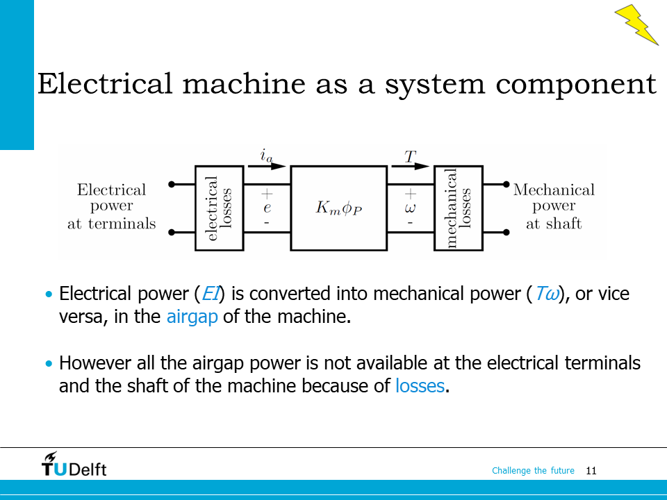
We may use the block diagram shown on the slide to represent an electrical machine operating in a system. The electrical machine takes electrical power from the electrical terminals, convert it to the mechanical power using magnetic field in the air gap of the machine, which is represented as the developed power.

However, not all electrical power is converted to mechanical power. There are always losses in the electrical and the mechanical sides, as we studied in the last lecture.

21.3. Control of a separately excited DC machine#

Now let us move on to study how a separately excited DC machine can be controlled with modern power electronics.

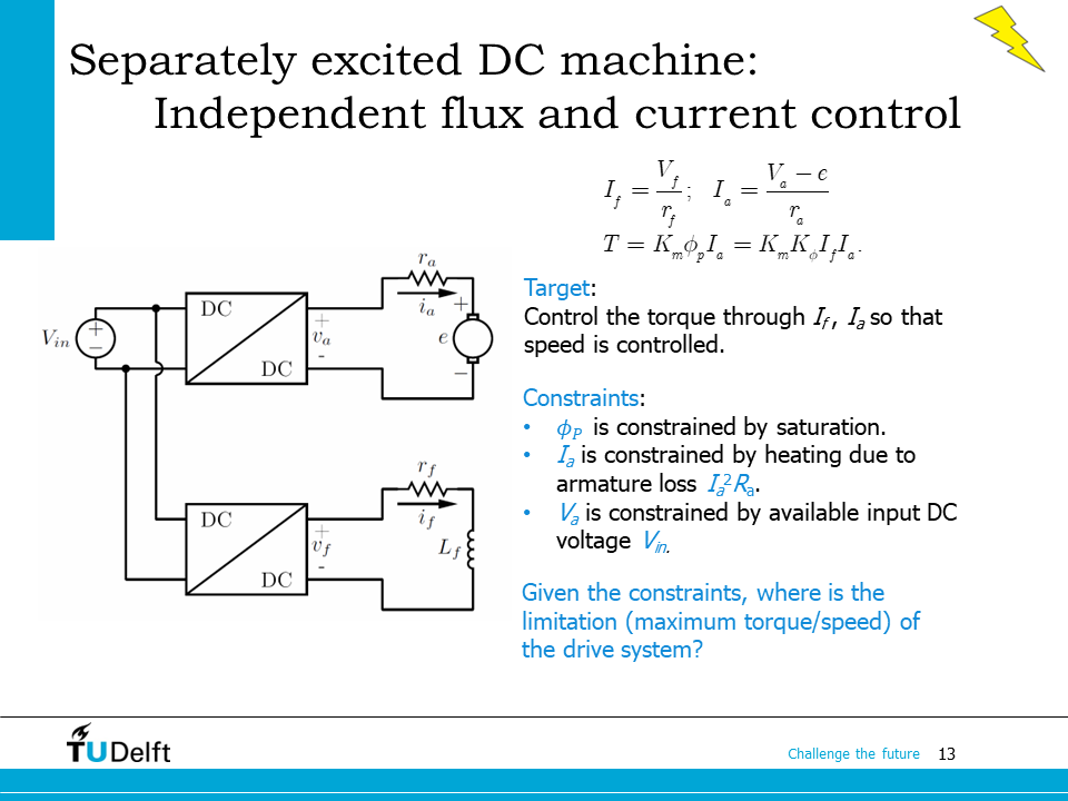
We may use two separate DC-DC converters to regulate the currents in the field circuit and the armature circuit independently. The steady state mathematical model of the system can be described as

\[\begin{split} \begin{align} I_f &= \frac{V_f}{r_f}, \quad \text{for the field circuit}; \\ I_a &= \frac{V_a-e}{r_a}, \quad \text{for the armature circuit}; \\ T &= K_m \phi_P I_a = K_m K_\phi I_f I_a, \quad \text{for the torque production}. \end{align} \end{split}\]

As we can see, the torque of the machine can be controlled by regulating \(I_f\) and \(I_a\).

However, \(I_f\) and \(I_a\) are not arbitrarily chosen, there are several constraints, as listed below:

The flux per pole \(\phi_P\) is constrained by the saturation in the magnetic core materials;
\(I_a\) is limited by temperature rise caused by the armature copper loss \(I_a^2r_a\) and cooling capability;
\(V_a\) is limited by the output capability of the DC-DC converter.

It is important to study where is the operation limit of the DC drive system considering the constraints above.

We will see how the control of a separately excited DC machine should adapt to maximise its operation limit in the coming slides.

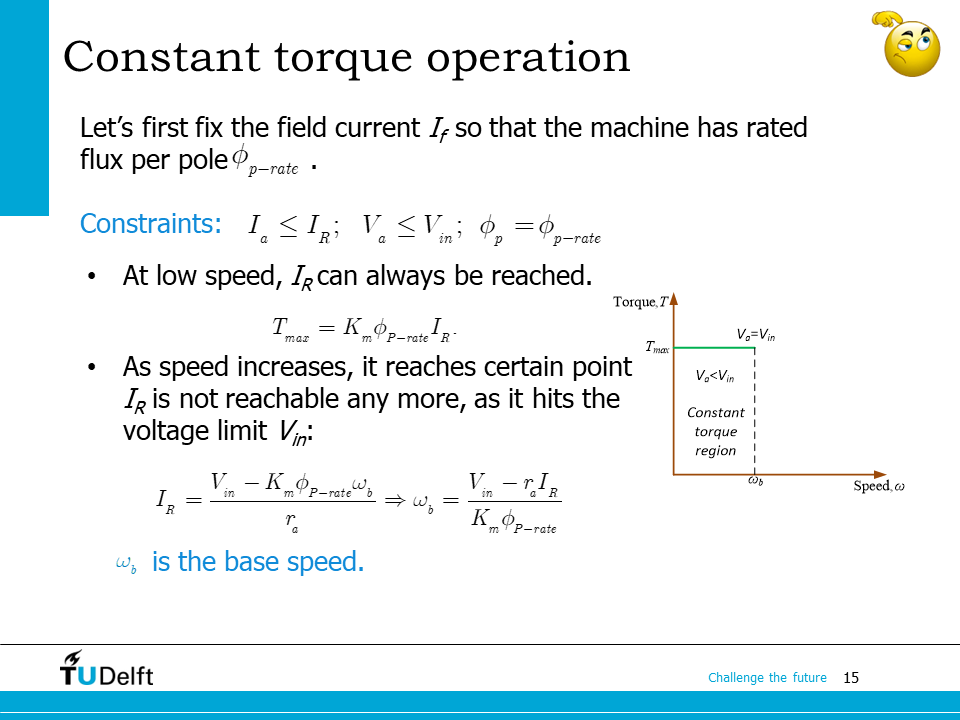
First we assume the field current is of the rated value, so that the machine has the rated flux per pole, and we only concern the forward motoring operation here.

\[ \phi_P = \phi_{P-rate}. \]

Assume a step down converter is used so that the armature voltage is limited by the input voltage

\[ V_a \leq V_{in}. \]

The armature current should be below the rated current \(I_R\), limited by the temperature rise.

\[ I_a \leq I_R. \]

When the speed is low enough, \(V_a\) is sufficient to push the rated current \(I_R\) to the armature circuit. The torque limit would be a constant

\[ T_{max} = K_m\phi_{P-rate} I_R. \]

As speed increases, the induced voltage also increases. At a certain point, \(V_a\) reaches the maximum value \(V_{in}\) to have the rated armature current. Afterwards, the armature current will drop because of insufficient armature voltage. The speed at this turning point is called the base speed, and is noted as \(\omega_b\). Based on the steady state equations, we know at the base speed,

\[ I_R = \frac{V_{in} - K_m\phi_{P-rate}\omega_b}{r_a}, \]

so the base speed is solved as

\[ \omega_b = \frac{V_{in}-r_aI_R}{K_m\phi_{P-rate}}. \]

The operation region between \(0\) to \(\omega_b\) is called the constant torque region, because the maximum torque is a constant, and the machine is able to achieve any torque below \(T_{max}\) at any speeds in this region.

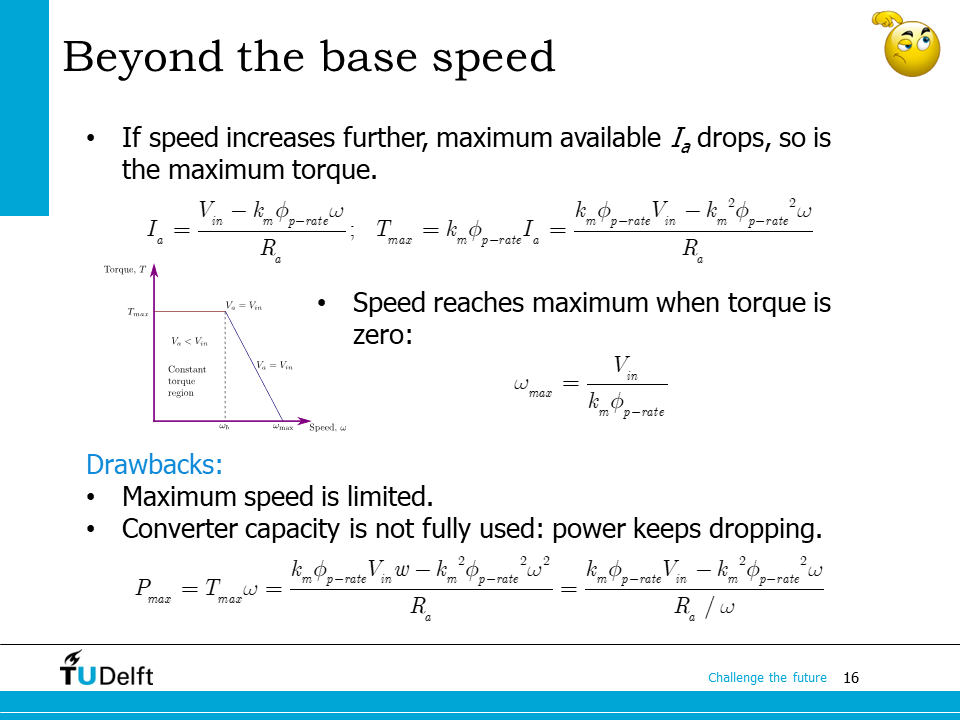
If the speed increases further beyond the base speed \(\omega_b\), the maximum available armature current will drop below \(I_R\), which becomes

\[ I_a = \frac{V_{in}-K_m\phi_{P-rate}\omega}{r_a}. \]

The maximum torque is then calculated as

\[ T_{max} = K_m\phi_{P-rate}I_a = \frac{K_m\phi_{P-rate}V_{in}-K_m^2\phi_{P-rate}^2\omega}{r_a}. \]

As we can see, the torque drops as \(\omega\) increases. When the speed drops to zero, the speed reaches the maximum value, which is solved from the equation above by setting \(T_{max} = 0\):

\[ \omega_{max} = \frac{V_{in}}{K_m\phi_{P-rate}}. \]

The maximum developed power we can obtain is derived from the maximum torque at specific angular speed

\[\begin{split} \begin{align} P_{max} &= T_{max}\omega = K_m\phi_{P-rate}I_a\omega \\ &= \frac{K_m\phi_{P-rate}V_{in}}{\omega r_a}-\frac{K_m^2\phi_{P-rate}^2}{ r_a}. \end{align} \end{split}\]

Apparently, the maximum power drops as speed increases.

This way of controlling the DC machine beyond the base speed has two drawbacks:

The machine is not able to operate beyond \(\frac{V_{in}}{K_m\phi_{P-rate}}\).
The power capacity of the converter is not sufficiently used, since the power drops as speed increases.

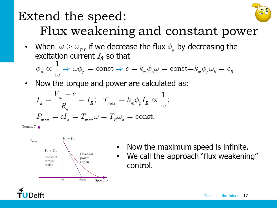
To further extend the speed and power limit when the speed is above the base speed, we could consider to limit the induced voltage, so that the rated current can still be pushed into the armature circuit. It can be achieved by reducing the flux per pole \(\phi_P\) by decreasing the excitation current \(I_f\).

If we reduce \(\phi_P\) so that it is inversely proportional to the angular speed, we will see that the induced voltage would become a constant:

\[\begin{split} \begin{align} e &= K_m\phi_P\omega = K_m \phi_{P-rate}\omega_b \\ &= e_R = \text{const}, \end{align} \end{split}\]

which stays at the rated value, the same as that of the base speed point.

Now the maximum armature current, torque, and power is calculated as

\[ I_a = \frac{V_{in}-e_R}{r_a} = I_R; \]

\[ T_{max} = K_m\phi_P I_R = \frac{e_RI_R}{\omega}; \]

\[ P_{max} = eI_a = e_RI_a = T_R\omega_b = \text{const}. \]

If we plot the \(T_{max}-\omega\) curve now, it will become a hyperbola curve when \(\omega>\omega_b\), as shown by the green curve on the slide. The maximum speed becomes infinite.

Moreover, the maximum power becomes a constant, which is the same as the power at the base speed. Therefore, the machine is able to achieve any power below \(P_{max}\) at any speeds in the \(\omega>\omega_b\) region, which is called the constant power region.

The control approach here is called “flux weakening” or “field weakening” since it reduces the flux per pole as speed increases above the base speed. Compared to the non-field-weakening approach, it has two advantages:

The maximum speed is increased;
The maximum deliverable power is increased and maintained as a constant at high speed.

Attention

Although in the theoretical analysis above, the maximum speed for field weakening operation and the constant power region is infinite, it is not achievable in practice because of many factors:

The duty cycle of the field winding converter;
The mechanical strength of the rotor;
The mechanical losses, brush losses etc.

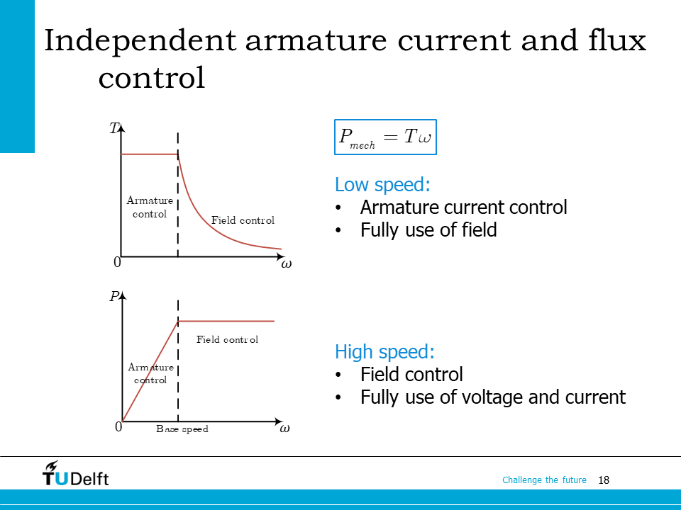
Now we plot the \(T-\omega\) and \(P-\omega\) curves as we analysed above. It can be seen that, when the speed is lower than the base speed, we keep field current constant, and control the armature current to regulate the torque. In this way, the magnetic field is sufficiently used.

When the speed is higher than the base speed, in addition to armature control, we also use field control to maintain the induced voltage as a constant value. During this process, the available voltage and current from the converter is sufficiently used.

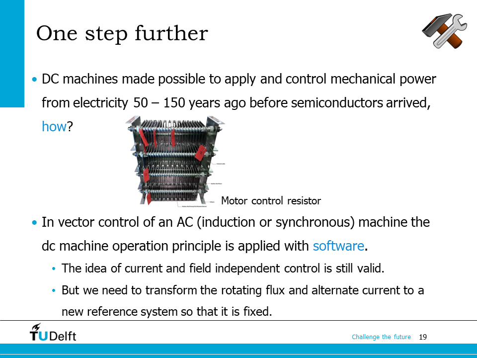
As we mentioned before, the motor drives have evolved in the last 150 years. In the beginning, we use motor control resistors and DC motors to make the electric drive system. After power semiconductors is invented, we can rely on power converters to make DC drives.

In practice, AC drives are more frequently used, because of its higher power density and reliability. However, the control principle of AC drives is the same as we learn here. We first convert the AC machine to a virtual DC machine in software, then apply the field control and armature control separately.

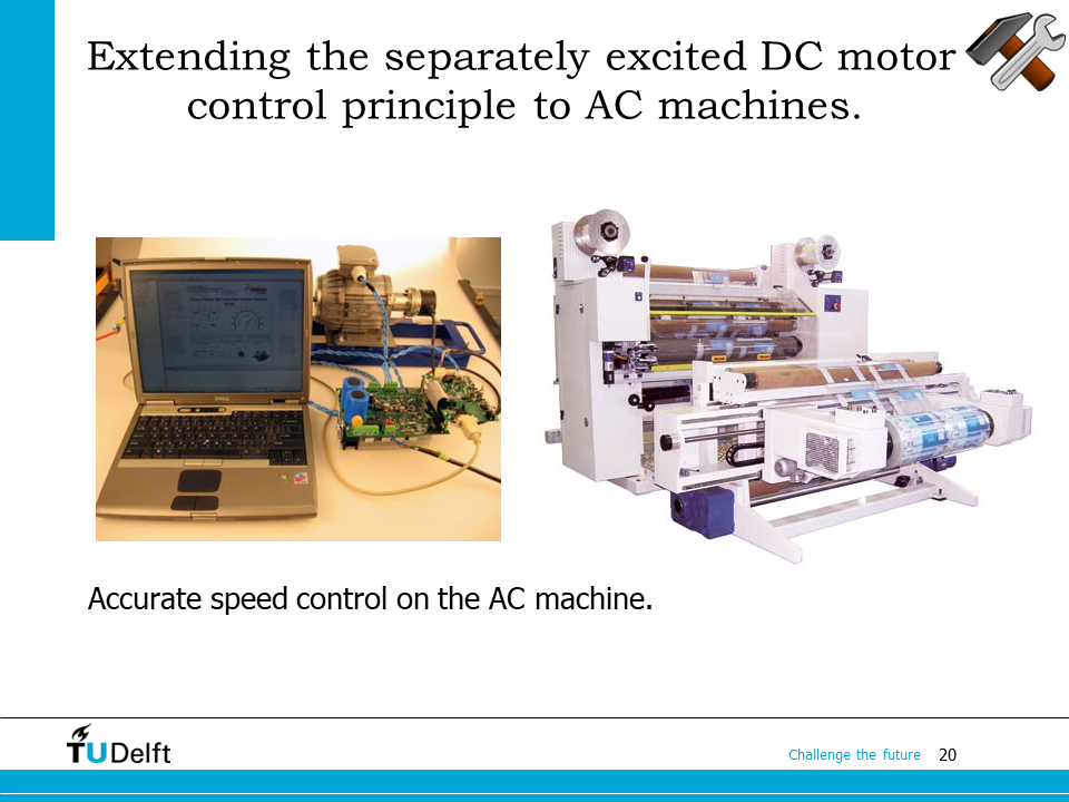
Here it shows an example of an AC machine based servo system.

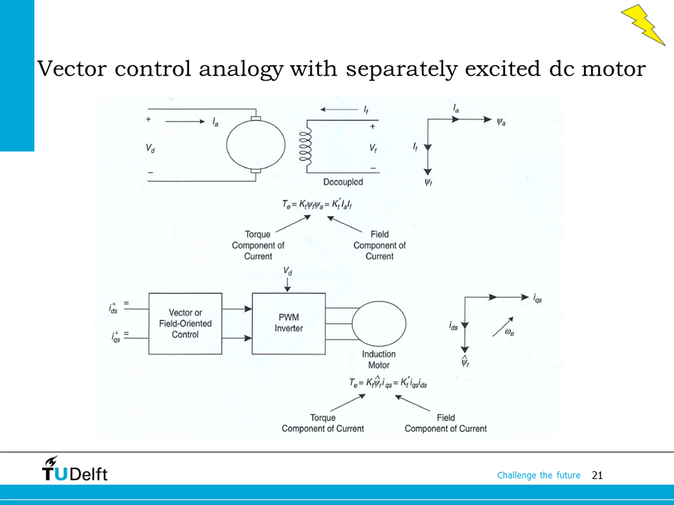
Here it shows the analogy between the separately excited DC motor and an induction machine. By applying field oriented transformations, the induction machine is first transformed to a virtual DC machine in software, so that the field and the torque can be controlled in a decoupled way. This will be further studied in the AC drives part of the course.

21.4. Converters in DC drives#

The next topic is how to use converters to realise the control principle we have discussed above.

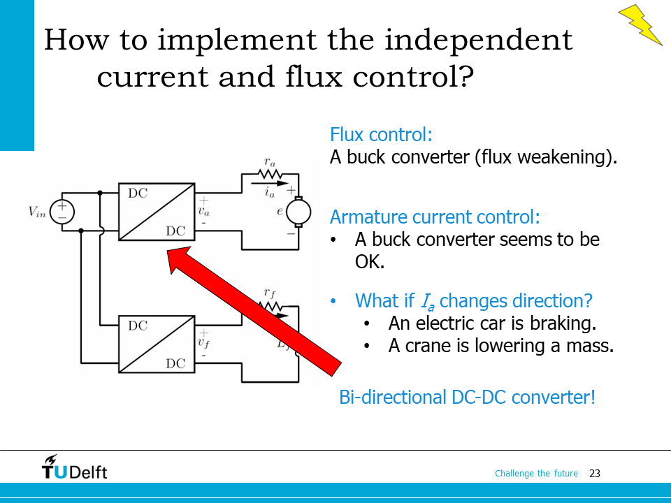
For the field circuit, a buck converter is sufficient, since we only need to do flux weakening (reducing field circuit voltage) at higher speed.

For the armature circuit, depending on its operation quadrants we may need bi-directional DC-DC converters, or 4-quadrant converters, since both the current and the rotation may change their directions.

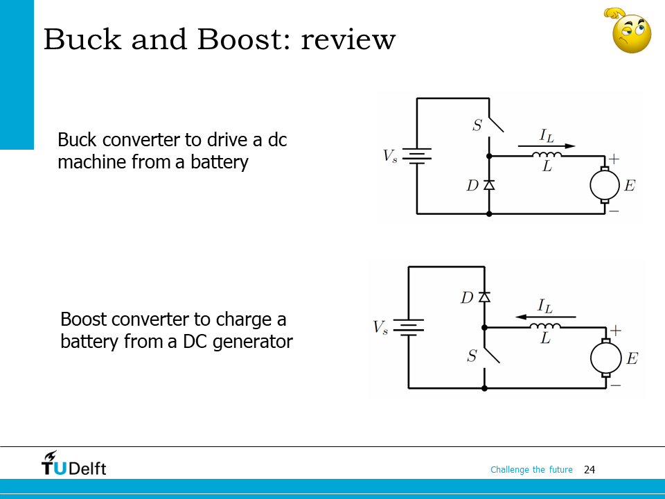
Let us first review how a bi-directional converter is constructed. By connecting a buck converter and a boost converter in parallel, we would be able to obtain a bi-directional converter.

When the power flows from the source to the DC machine, it operates in the buck mode. Otherwise, it operates in the boost mode.

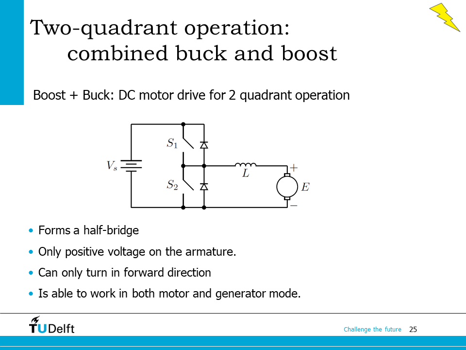
The bi-directional DC-DC converter is in essence a 2-quadrant converter. It is also called a half bridge, which is the basic building block of more complicated power electronics converters.

The converter is only able to have positive output voltage, so the DC machine connected to it can only turn in the forward direction, but since the current is reversible, it is able to operate the DC machine in both forward motoring and forward braking mode.

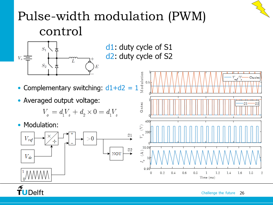
In practice, we usually use the pulse-width-modulation method to regulate the half bridge. The two switches \(S_1\) and \(S_2\) are switched in a complementary way, i.e., when \(S_1\) is on, \(S_2\) is off, or vice versa. The average output voltage can be calculated as \(\bar{V}_o = d_1 V_s\).

What you see on the slide is the block diagram and the waveforms to show how the pulse width modulation is realised using a triangular carrier waveform.

21.5. Four-quadrant operation#

In many cases, i.e., a car or a crane, the rotation should happen in both ways. Then it requires 4-quadrant operation of DC machines.

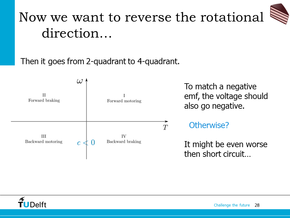
To match the negative induced voltage (or electromotive force, EMF) caused by backward rotation, the input voltage should also go negative, otherwise the machine will not operate properly, and the machine and the converter may even be destroyed by large current.

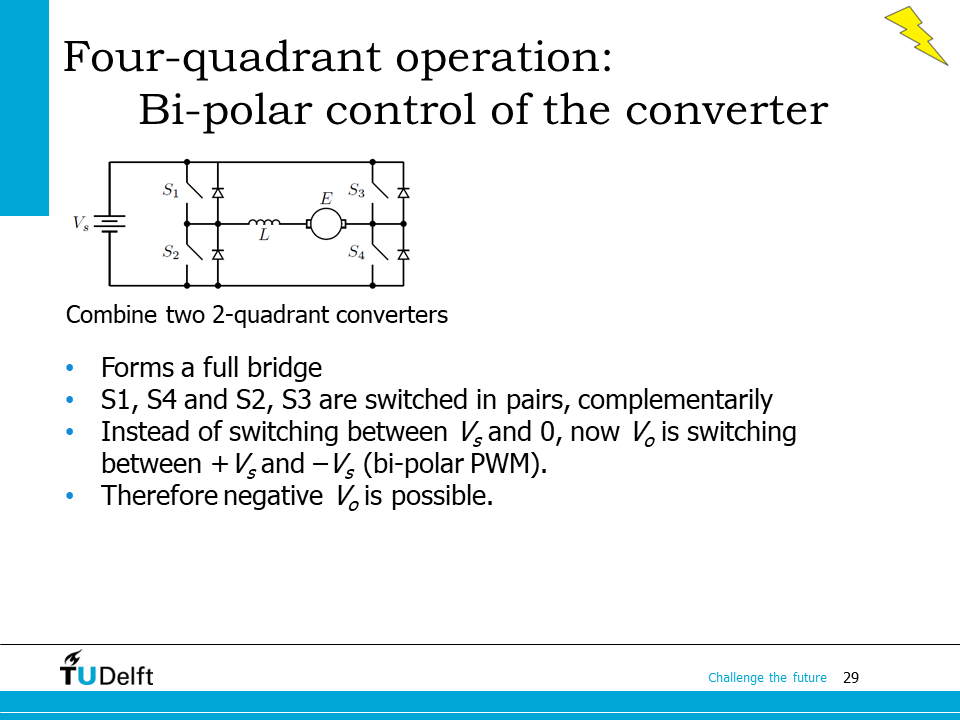
A 4-quadrant converter can be obtained by combining two 2-quadrant converters (half bridges) as shown on the slide. This topology is also called a full bridge, which is able to deliver both positive and negative output voltage.

There are two ways to modulate the four-quadrant converter. The first one is called bipolar modulation, where \(S_1\), \(S_4\) and \(S_2\), \(S_3\) are switched in pairs and in a complementary way. When \(S_1\) and \(S_4\) are on, \(V_s\) is obtained on the terminal of the DC machine. When \(S_2\) and \(S_3\) are on, \(-V_s\) is obtained on the terminal of the DC machine. When pulse-width modulation is used, the output voltage is switched between \(V_s\) and \(-V_s\), that’s why it is called bipolar PWM.

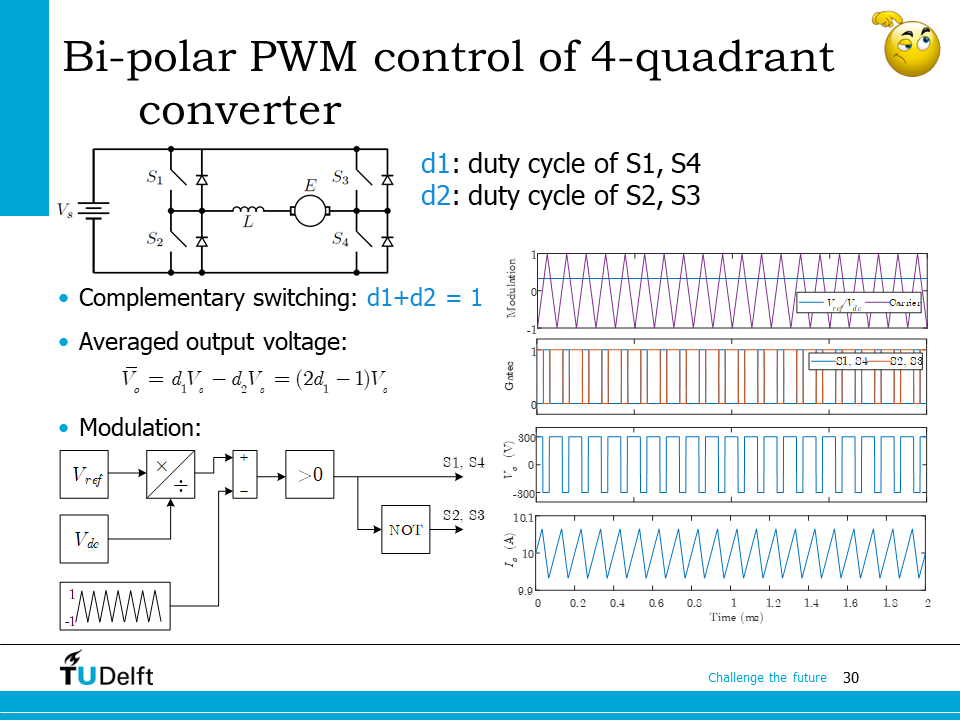
This slide shows the block diagram and the triangular carrier waveform based bipolar PWM method of the 4-quadrant converter. The average output voltage can be related to the duty cycles by

\[ \bar{V}_o = d_1V_s - d_2V_s = (2d_1-1)V_s. \]

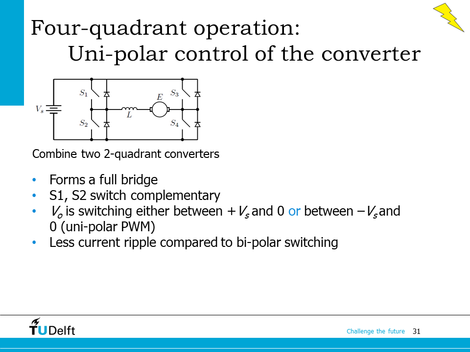
A second way to modulate the 4-quadrant converter is the unipolar modulation. As the name indicates, the output of the converter is switched either between \(V_s\) and 0, or between \(-V_s\) and 0. This is done by generating the positive half of the reference voltage in from left half bridge, and the negative half of the reference voltage from the right half bridge.

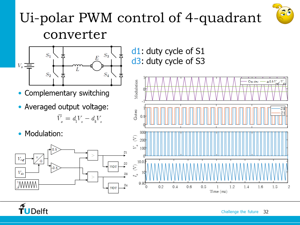
This slide shows the block diagram and the triangular carrier waveform based unipolar PWM method of the 4-quadrant converter. The average output voltage can be related to the duty cycles by

\[ \bar{V}_o = d_1V_s - d_3V_s. \]

As we can see from the waveform, \(V_{ref}/2\) is generated from the left half bridge, while \(-V_{ref}/2\) is generated from the right half bridge. The output is only switching between 0 and \(V_s\) (or 0 and \(-V_s\) if the reference is a negative voltage), therefore, compared to the bipolar modulation, it delivers less voltage and current ripples.

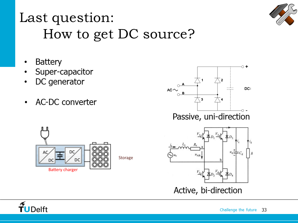
The last question to be answered for the DC drive is where the DC source comes from. In electric car applications, batteries are often used.

In industrial or household applications, DC power is often obtained by rectifying the AC power. The power converter to convert AC power to DC power is called a rectifier. Based on whether active semiconductors or passive semiconductors (diodes) are used, they can be classified into active rectifiers and active rectifiers.

Only the active rectifier can enable bi-directional power flow between AC and DC, so in applications like V2G (vehicle to grid), a active rectifier is needed.

21.6. Homework#

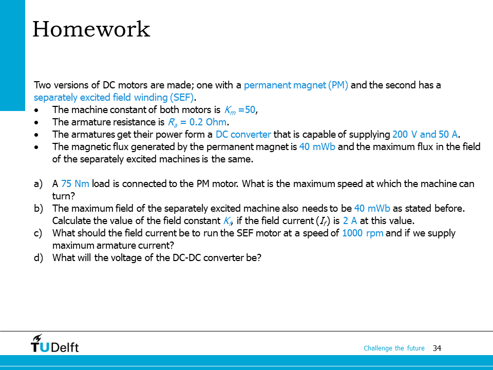
The homework is for you to practice the calculation of DC drive performances.

Please first try to work it out yourself, and click the hidden content below to check your answer.

a) The maximum speed is 919.120 rpm.
b) The field constant is 0.020 H.
c) The field current is 1.500 A.
d) The voltage of the DC-DC converter is 167.080 V.