22. AC Machine Stator

The last part of the course is on AC machines. The two main types of AC machines will be studied: the synchronous machine and the induction machine. We will start with the stator part of the AC machines, since both the synchronous machine and the induction machine have the same type of stator.

After taking this lecture, we should be able to tell the construction of the stator of an AC machine, understand how a rotating magnetic field is generated from three phase windings, and how the rotating field leads to three phase induced voltage. Afterwards, we wills study how the mechanical rotating speed can be varied by changing the number of poles.

22.1. AC machine stator structure

We first take a look at the structure of AC machines.

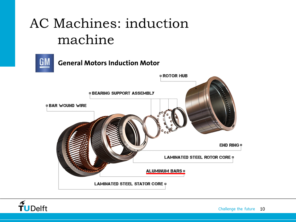
The picture here shows the exploded-view of an induction machine. As we can see, the stator part has a magnetic core made of laminated steel sheets staking together. There are three phase coils inserted into the slots punched on the stator lamination. The rotor side also has a laminated structure. However, aluminium bars are inserted into the rotor slots instead of coils. The rotor bars are shorted together by the end rings on both ends of the rotor. In high performance applications, the rotor bar can also be made from copper.

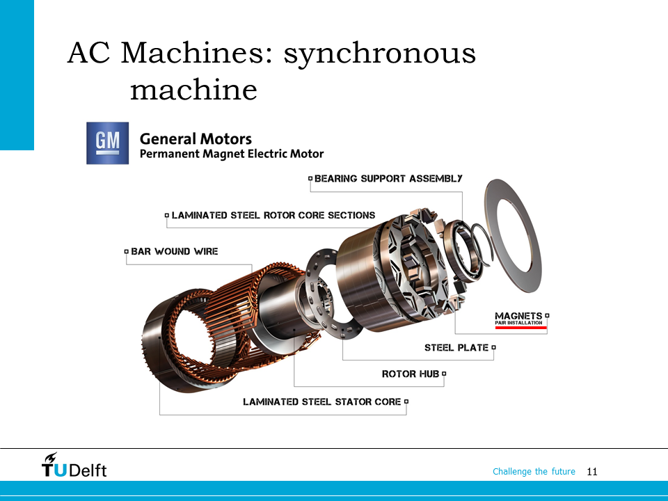
Here it shows the exploded-view of a synchronous machine. The stator has the same structure: a laminated steel stator core, with three phase coils inserted into the slots. The rotor is however different from that of the induction machine. Permanent magnets are inserted to the rotor slots instead of conductor bars. It is also possible to use electromagnets to replace the permanent magnets to make a synchronous machine.

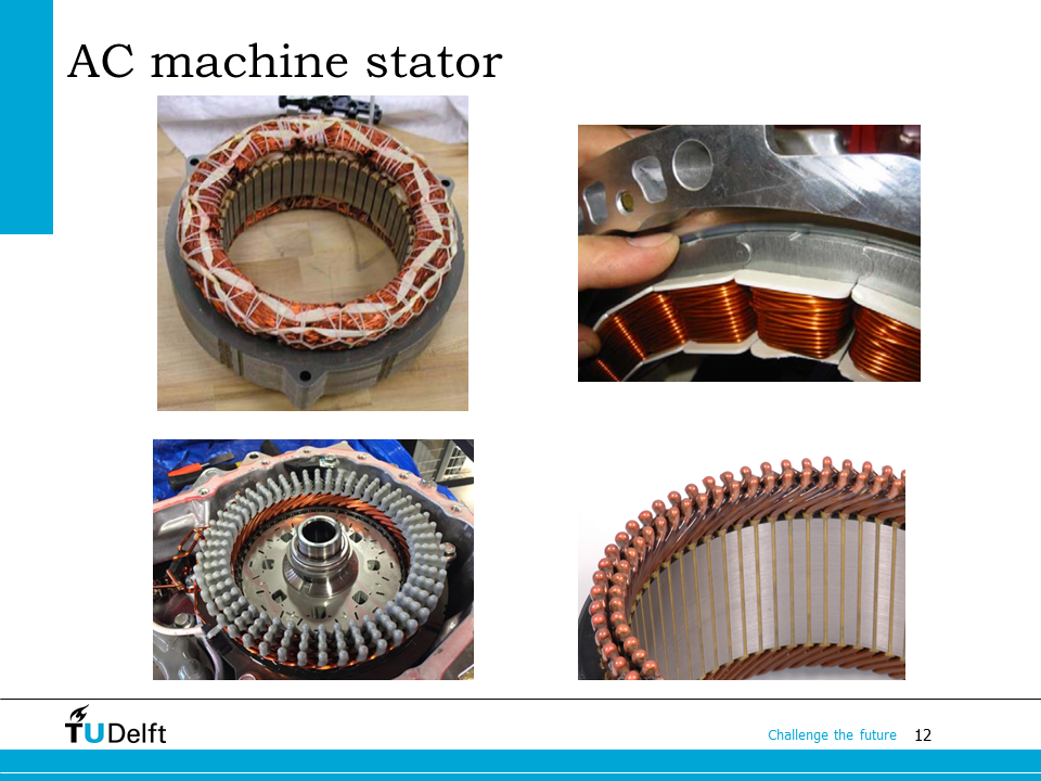
Here it shows several examples of the AC machine stator. On the top left, the winding is spanning in the stator slots. Round wires are used to form the winding.

On the top right, each coil is wounded around each stator tooth. We can call the winding single-pitch winding.

In the bottom figures, the winding is made of bars shaped like hairpins, therefore, it is also called hairpin winding. The hairpin winding can achieve high pack factor (the ratio between the total copper cross sectional area versus the total slot area in one slot), so that it is often used in applications which require high power density, e.g. electric vehicle traction motors.

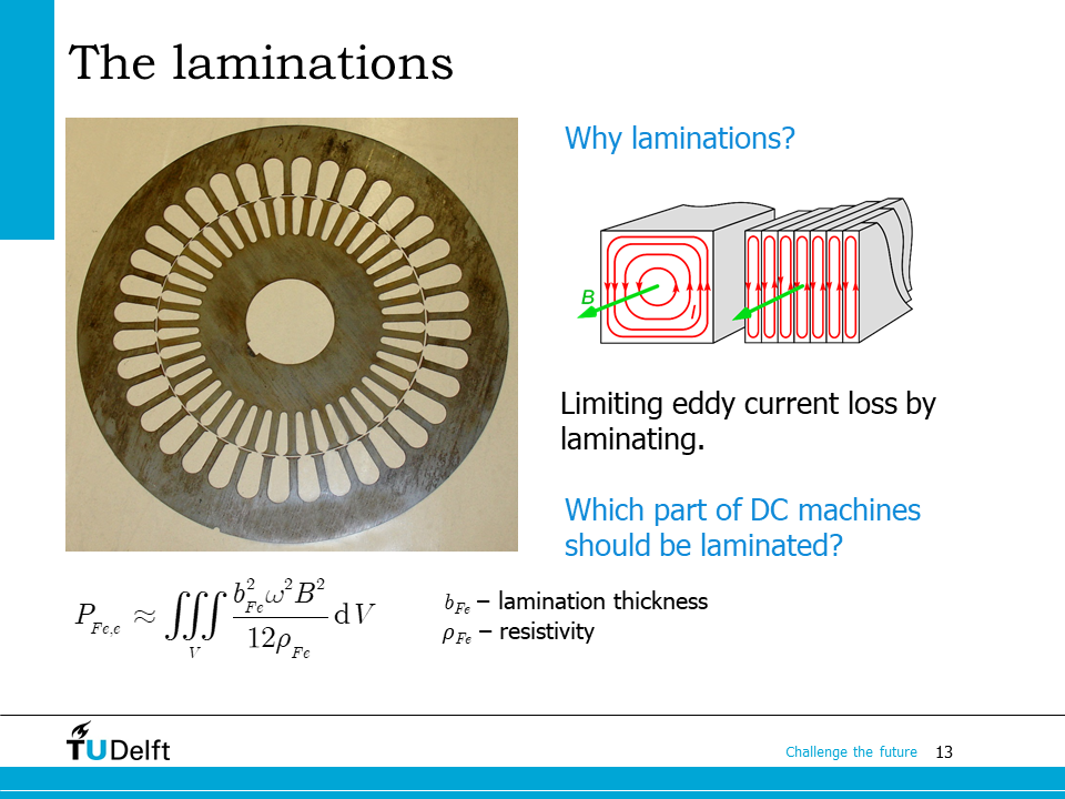
On the slide you can see the rotor and stator laminations of an induction machine. Between them there is a small gap between them, which is called air gap, so that the rotor can rotate and the magnetic flux can flow through. There are slots punched on the laminations. The slots can be used to place the coil or conductor bars. The parts between adjacent slots are called teeth.

We have already studied in the magnetic part of the course that there will be eddy current and eddy current loss inside the magnetic core. By laminating the magnetic core, the eddy current paths inside the silicon steel sheets will be increased, so that for the same flux density, the eddy current and the loss caused by it will be suppressed.

For a DC machine, the rotor part of the DC machine has to be laminated, since it experiences a rotating magnetic field as rotor rotates. The stator core can be a solid one, since the main field is fixed. However, inside a universal machine (a series wound DC machine), the stator is also laminated, since we can feed an universal machine with AC voltage.

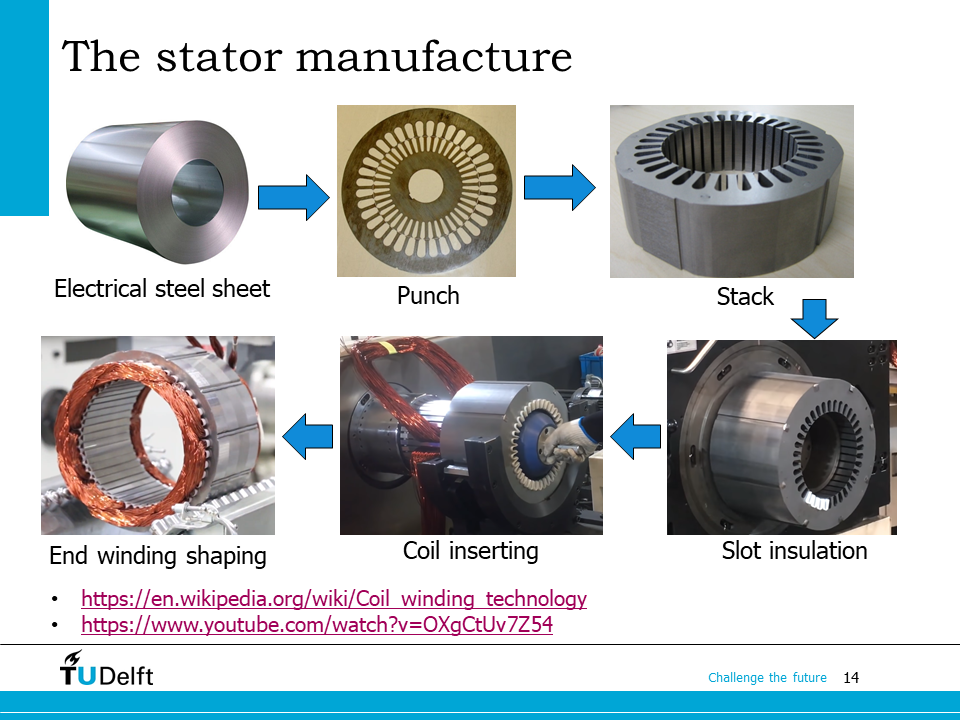
The manufacturing process of the AC machine stator is shown on the slide. The electrical steel sheet is usually delivered in the form of coils. We first cut it to the required size, then punching or cutting machines are used to make the slots on the silicon steel sheets. The punched laminations are stacked together to form a magnetic core. Then slot insulation is inserted to the slots to protect the coils. The coils are then inserted to the slots to form a winding. In the end, the ends of the winding will be shaped, and additional end-winding insulation will be applied. You may find additional information regarding stator winding manufacturing here. The video below demonstrates the process abov.

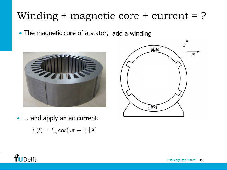
Once we have a magnetic core and a winding, by applying current into the winding, a magnetic field will be generated based on Ampere’s Law.

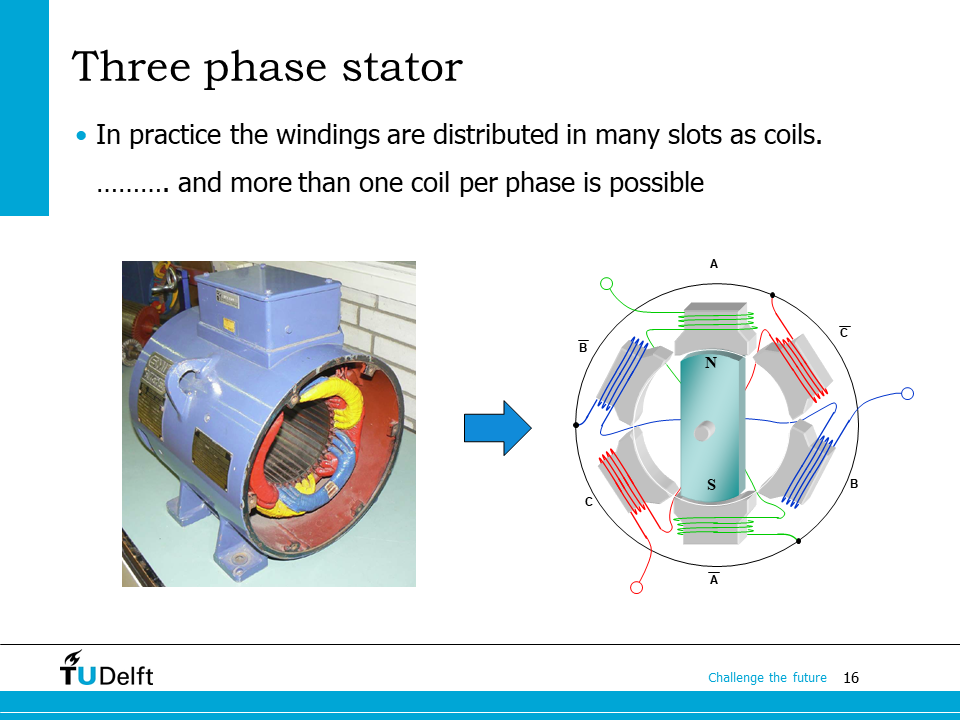
In practice, the stator winding is always distributed in many slots. The coils in the slots are inner-connected to form a winding. Here it shows a three-phase winding and its simplified schematic on the right.

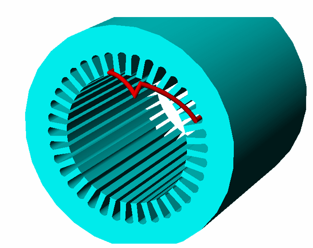
The animation below shows how a three phase winding is constructed by inserting coils into slots.

22.2. Magnetic flux density in the air gap

Let’s first study the magnetic flux density generated from one phase winding.

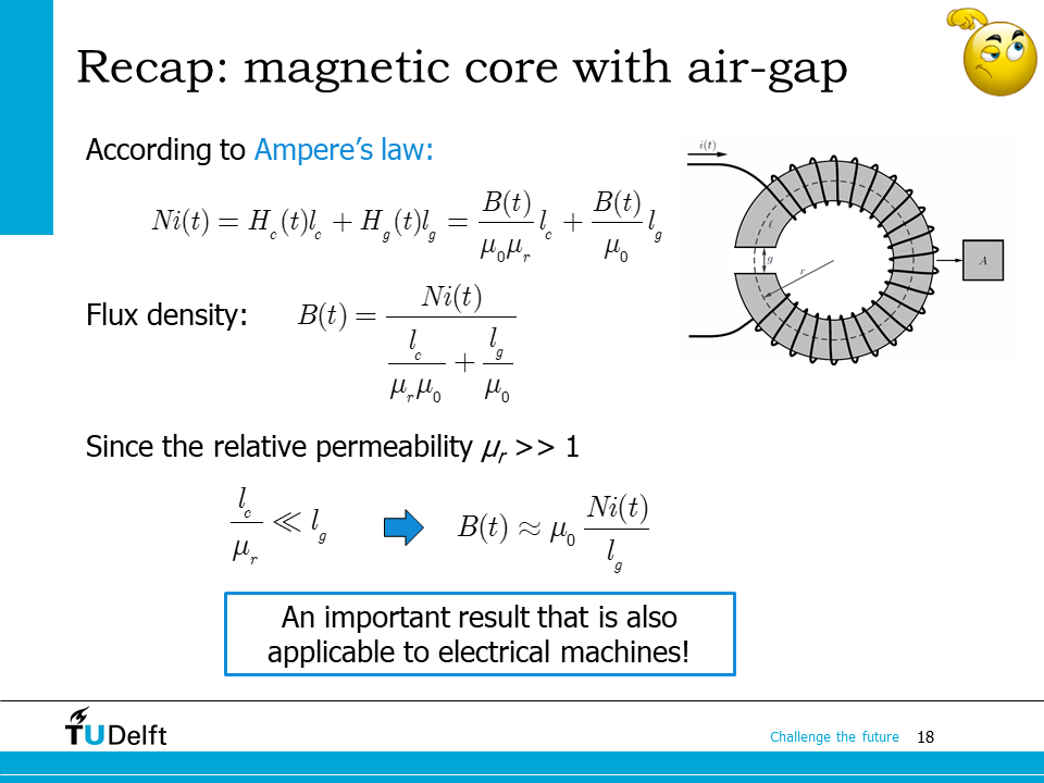
Here it recalls the Ampere’s law which can be applied to solve the flux density inside the air gap of an electrical machine. When a coil is wound around a magnetic core, if the permeability is sufficiently high, the flux density inside the air gap can be approximated by

\[ B \approx \mu_0\frac{Ni(t)}{l_g}. \]

We will apply the same principle to analyse the magnetic field inside the electrical machine.

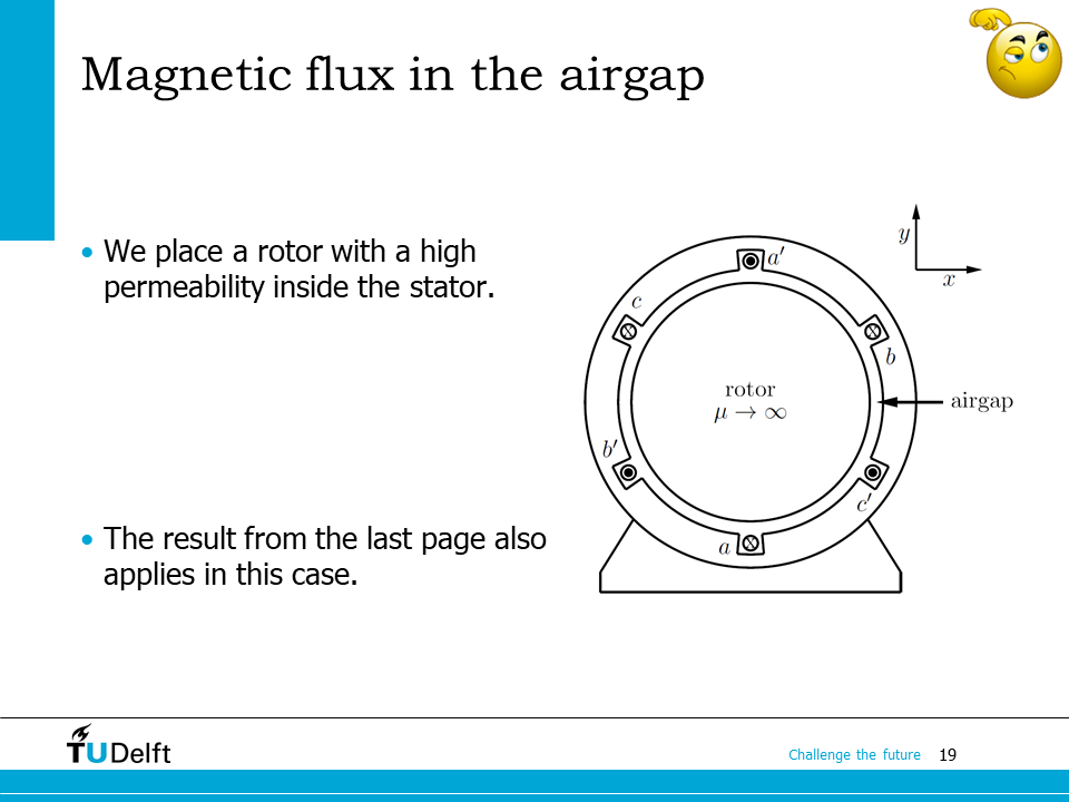
Let us assume the permeability inside the stator and the rotor core are infinitely high, and the slot width is negligible. The three phase windings are displaced by 120 degree from each other. We also assume that all the winding sides concentrate on a single point with negligible width on the surface of the stator.

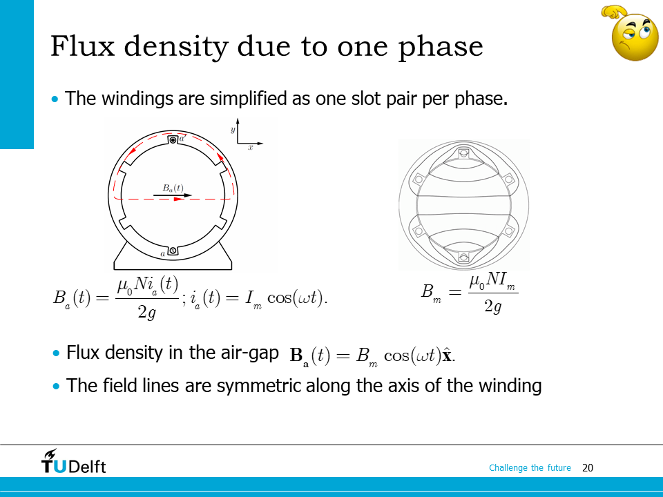
If the number of turns for each phase winding is \(N\), the current in phase a is \(i_a(t) = I_a \cos(\omega t)\). By applying the Ampere’s law, we know the magnetic flux density generated by phase a is

\[ B_a(t) = \frac{\mu_0 N i_a(t)}{2g} = \frac{\mu_0 N I_m\cos(\omega t)}{2g}. \]

where \(g\) is the air gap length.

We can see the flux density is alternating by time, and the flux lines are symmetric along the axis of the winding. Let us define the amplitude of this flux density as \(B_m\).

\[ B_m = \frac{\mu_0 N I_m}{2g}. \]

Using vector notation, we know the flux density vector is

\[ \mathbf{B_a}(t) = B_m\cos(\omega t) \hat{\mathbf{x}} \]

since the flux lines are symmetric along the axis of the winding, i.e., the x-axis. Here \(\hat{\mathbf{x}}\) is the unit direction vector of the x-axis.

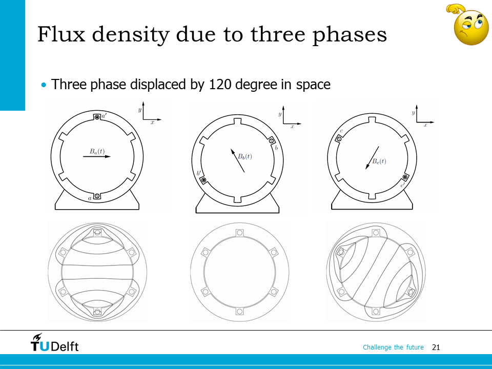
Similarly, we are able to obtain the flux density generated from phase b and phase c:

\[\begin{split} \begin{align} B_b(t) &= \frac{\mu_0 N i_b(t)}{2g},\\ B_c(t) &= \frac{\mu_0 N i_c(t)}{2g}. \end{align} \end{split}\]

22.3. Rotating magnetic field

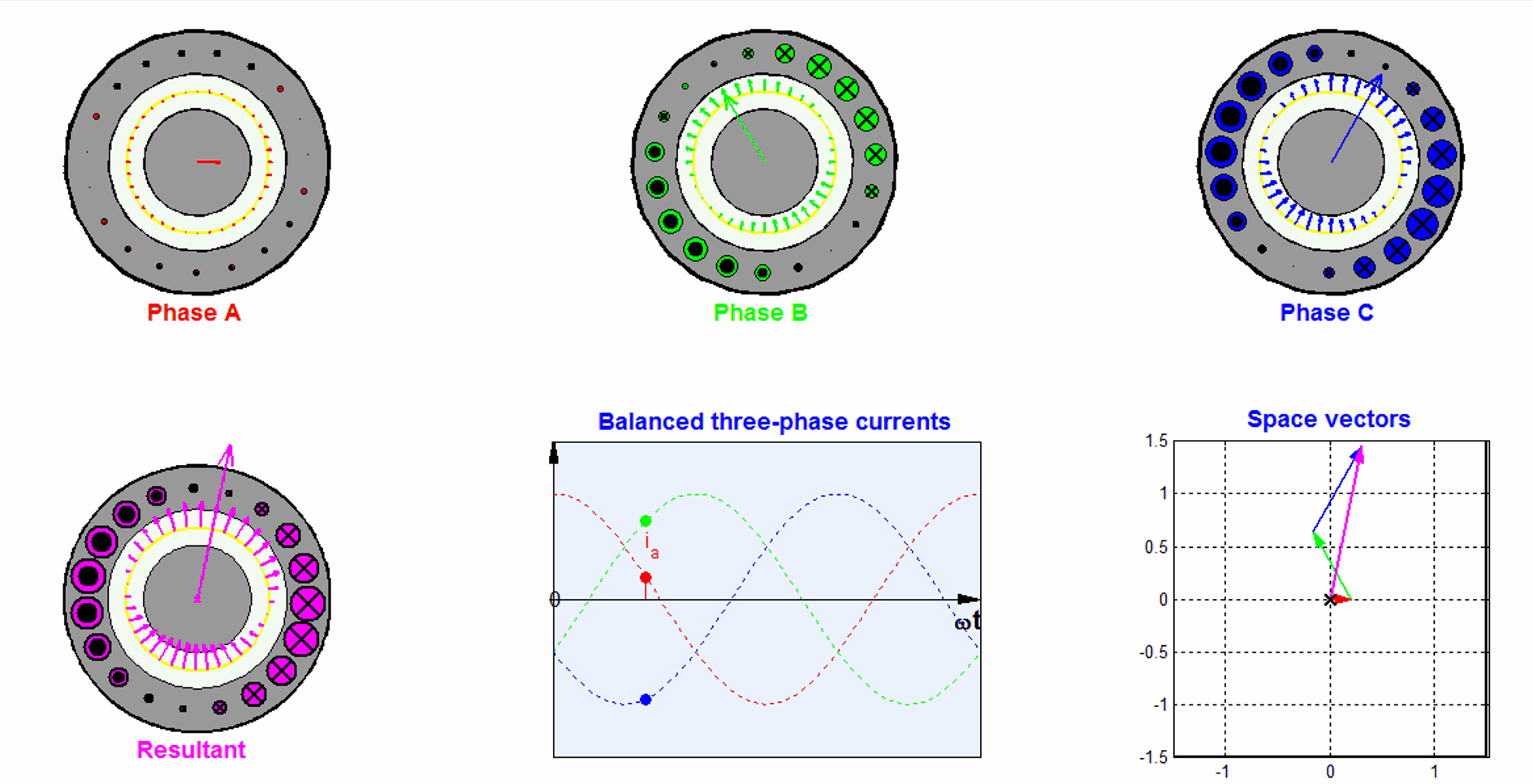
Now let us investigate the case when all three phase currents are applied to the winding.

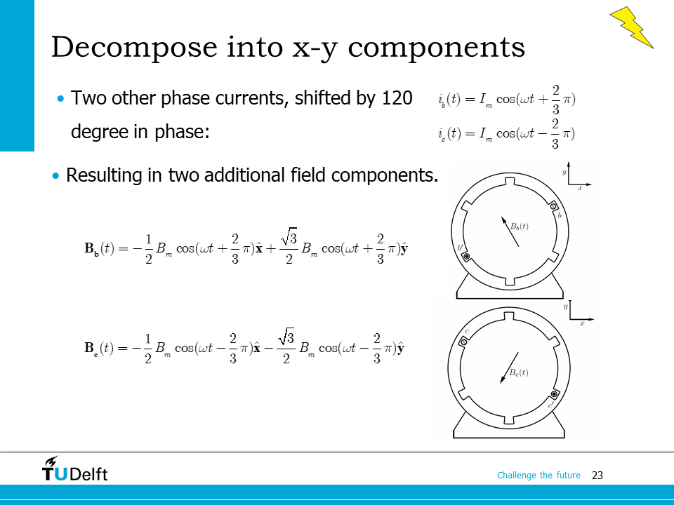
Let us assume a symmetric three phase, and the phase sequence of a-c-b, i.e., all three phase currents have the same amplitude, and phase c lags phase a by \(\frac{2\pi}{3}\) in phase, and phase b lags phase c by \(\frac{2\pi}{3}\) in phase. Because of the spatial position of phase b and phase c, we could derive the flux density vectors generated from phase b and c, by decomposing them into the x and y components

\[\begin{split} \begin{align} \mathbf{B_b}(t) &= B_b(t)\cos(\frac{2\pi}{3}) \hat{\mathbf{x}} + B_b(t)\sin(\frac{2\pi}{3}) \hat{\mathbf{y}}\\ &= -\frac{1}{2}B_m\cos(\omega t+\frac{2\pi}{3}) \hat{\mathbf{x}}+\frac{\sqrt{3}}{2}B_m\cos(\omega t+\frac{2\pi}{3}) \hat{\mathbf{y}} \\ \mathbf{B_c}(t) &= B_c(t)\cos(\frac{-2\pi}{3}) \hat{\mathbf{x}} + B_c(t)\sin(\frac{-2\pi}{3}) \hat{\mathbf{y}}\\ &= -\frac{1}{2}B_m\cos(\omega t-\frac{2\pi}{3}) \hat{\mathbf{x}}-\frac{\sqrt{3}}{2}B_m\cos(\omega t-\frac{2\pi}{3}) \hat{\mathbf{y}} \\ \end{align} \end{split}\]

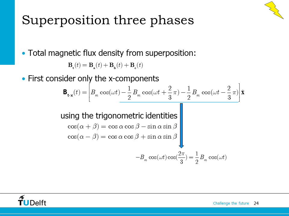
The total magnetic flux density can be obtained by superimposing the contributions from all three phases.

\[ \mathbf{B_t}(t) = \mathbf{B_a}(t)+\mathbf{B_b}(t)+\mathbf{B_c}(t). \]

The x-component of \(\mathbf{B_t}(t)\) is then

\[ \mathbf{B_{t-x}}(t) = \left[ B_m\cos(\omega t)-\frac{1}{2}B_m\cos(\omega t+\frac{2\pi}{3})-\frac{1}{2}B_m\cos(\omega t-\frac{2\pi}{3}) \right] \hat{\mathbf{x}}. \]

By applying the trigonometric identities, the above equation can be simplified to

\[ \mathbf{B_{t-x}}(t) = \frac{3}{2}B_m\cos(\omega t) \hat{\mathbf{x}}. \]

Similarly, the y-component is

\[ \mathbf{B_{t-y}}(t) = -\frac{3}{2}B_m\sin (\omega t) \hat{\mathbf{y}}. \]

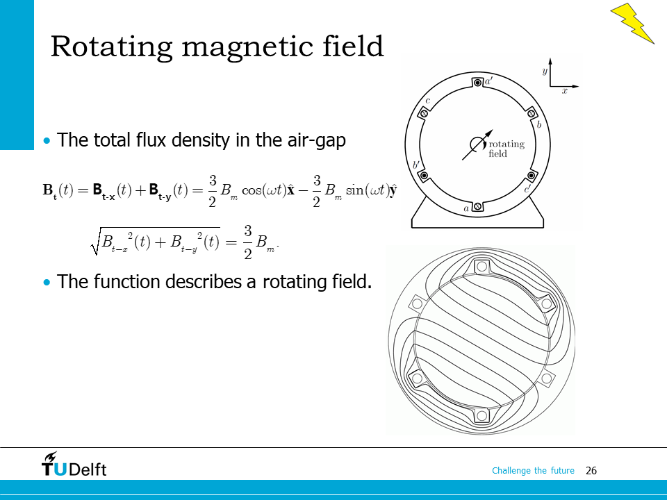
The total flux density vector is then

\[\begin{split} \begin{align} \mathbf{B_{t}}(t) &= \mathbf{B_{t-x}}(t) + \mathbf{B_{t-y}}(t) \\ &= \frac{3}{2}B_m\cos(\omega t) \hat{\mathbf{x}} -\frac{3}{2}B_m\sin (\omega t) \hat{\mathbf{y}}. \end{align} \end{split}\]

The trajectory of the flux density vector is a circle as \(t\) increases. So we can see the three phases together contribute to a rotating magnetic field, and the magnitude of the rotating flux density is 3/2 times that contributed from one single phase.

The script below derive the magnetic field generated from three phases and shows an animation to demonstrate the superposition from the three phase magnetic fields.

Show code cell source Hide code cell source

%reset -f
from sympy import *

t, I_m, N, g, mu_0 = symbols('t, I_m, N, g, mu_0')
omega = symbols('omega', positive=True)

i_a = I_m*cos(omega*t)
i_b = I_m*cos(omega*t + 2*pi/3)*exp(I*2*pi/3)
i_c = I_m*cos(omega*t - 2*pi/3)*exp(-I*2*pi/3)

B_a = mu_0*N*i_a/(2*g)
B_b = mu_0*N*i_b/(2*g)
B_c = mu_0*N*i_c/(2*g)

B_t = B_a+B_b+B_c

print('The total flux density generated from the three phases is:')
B_t=B_t.rewrite(cos)
simplify(B_t)

The total flux density generated from the three phases is:

\[\displaystyle \frac{3 I_{m} N \mu_{0} e^{- i \omega t}}{4 g}\]

Show code cell source Hide code cell source

import numpy as np
import matplotlib
matplotlib.rcParams['text.usetex'] = True
import matplotlib.pyplot as plt
plt.rcParams['figure.figsize'] = [4.5, 3]
plt.rcParams['figure.dpi'] = 200 # 200 e.g. is really fine, but slower
from matplotlib.animation import FuncAnimation
from IPython import display

B_t_subs = B_t.subs([(omega, 2*pi*50),(N, 100), (I_m, 10), (g, 0.001), (mu_0, 4*pi*1e-7)])
B_a_subs = B_a.subs([(omega, 2*pi*50),(N, 100), (I_m, 10), (g, 0.001), (mu_0, 4*pi*1e-7)])
B_b_subs = B_b.subs([(omega, 2*pi*50),(N, 100), (I_m, 10), (g, 0.001), (mu_0, 4*pi*1e-7)])
B_c_subs = B_c.subs([(omega, 2*pi*50),(N, 100), (I_m, 10), (g, 0.001), (mu_0, 4*pi*1e-7)])

B_t_fun  = lambdify(t, B_t_subs)
B_a_fun  = lambdify(t, B_a_subs)
B_b_fun  = lambdify(t, B_b_subs)
B_c_fun  = lambdify(t, B_c_subs)

fig, ax = plt.subplots()

def animate(t):
    ax.clear()
    ax.set_xlim(-1, 1.0)
    ax.set_ylim(-1, 1.0)
    ax.set_xlabel('$B_x$')
    ax.set_ylabel('$B_y$')
    ax.set_aspect('equal')
    Bt = B_t_fun(t)
    Ba = B_a_fun(t)
    Bb = B_b_fun(t)
    Bc = B_c_fun(t)
    plt.arrow(0, 0, Ba.real, Ba.imag, width = 0.01, color='r', length_includes_head=True, label='$B_a$')
    plt.text(Ba.real/2, Ba.imag/2, '$B_a$', color='r')
    plt.arrow(Ba.real, Ba.imag, Bb.real, Bb.imag, width = 0.01, color='g', length_includes_head=True, label='$B_b$')
    plt.text(Ba.real+Bb.real/2, Ba.imag+Bb.imag/2, '$B_b$', color='g')
    plt.arrow(Ba.real+Bb.real, Ba.imag+Bb.imag, Bc.real, Bc.imag, width = 0.01, color='b', length_includes_head=True, label='$B_c$')
    plt.text(Ba.real+Bb.real+Bc.real/2, Ba.imag+Bb.imag+Bc.imag/2, '$B_c$', color='b')
    plt.arrow(0, 0, Bt.real, Bt.imag, width = 0.01, length_includes_head=True, label='$B_t$')
    plt.text(Bt.real/2, Bt.imag/2, '$B_t$')
    plt.tight_layout()
    
anim = FuncAnimation(fig, animate, frames=np.linspace(0, 1.0/50, 200), interval=20)

video = anim.to_html5_video()
html = display.HTML(video)
display.display(html)
plt.close() 

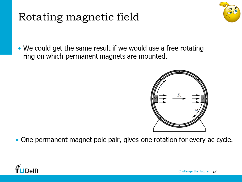
The same rotating magnetic field can also be generated by rotating permanent magnet pairs, as shown on the slide.

For one permanent magnet pair, every ac cycle (a period of the induced voltage) is corresponding to one revolution in space.

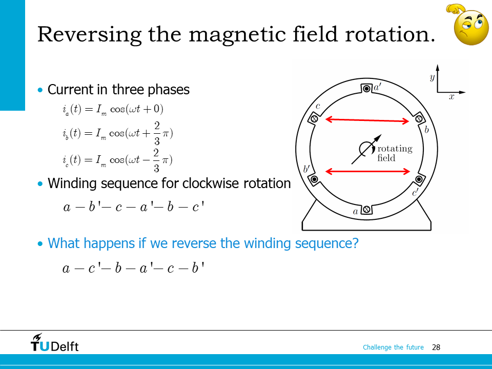
Be aware that the example we analysed before was with the phase sequence of a-c-b. If we reverse the phase sequence to a-b-c and keep the winding configuration, the rotational direction of the magnetic field will also be reversed.

In such case,

\[\begin{split} \begin{align} i_a(t) &= I_m \cos(\omega t)\\ i_b(t) &= I_m \cos(\omega t - \frac{2\pi}{3})\\ i_c(t) &= I_m \cos(\omega t + \frac{2\pi}{3}). \end{align} \end{split}\]

and

\[\begin{split} \begin{align} \mathbf{B_{t}}(t) &= \mathbf{B_{t-x}}(t) + \mathbf{B_{t-y}}(t) \\ &= \frac{3}{2}B_m\cos(\omega t) \hat{\mathbf{x}} +\frac{3}{2}B_m\sin (\omega t) \hat{\mathbf{y}}. \end{align} \end{split}\]

You may play with the scripts above to validate the result.

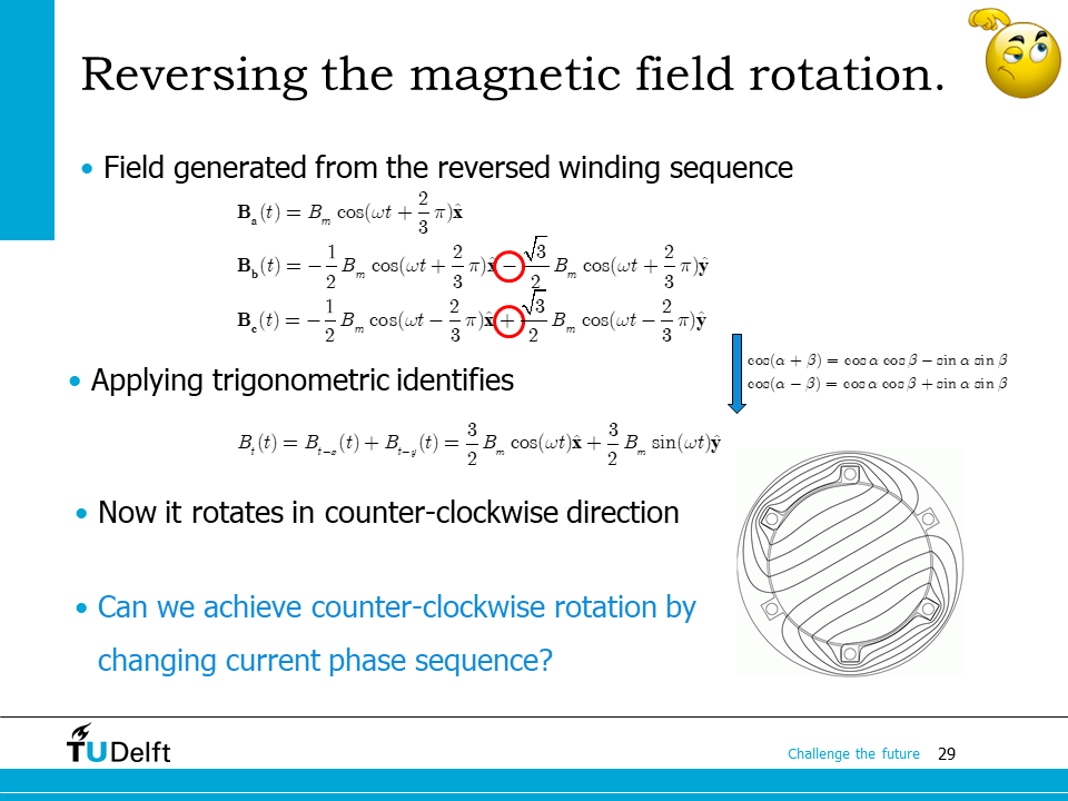
Similarly, if we keep the phase sequence the same, but swap the spatial position of phase b and phase c. Now,

\[\begin{split} \begin{align} \mathbf{B_b}(t) &= B_b(t)\cos(-\frac{2\pi}{3}) \hat{\mathbf{x}} + B_b(t)\sin(-\frac{2\pi}{3}) \hat{\mathbf{y}}\\ &= -\frac{1}{2}B_m\cos(\omega t+\frac{2\pi}{3}) \hat{\mathbf{x}}-\frac{\sqrt{3}}{2}B_m\cos(\omega t+\frac{2\pi}{3}) \hat{\mathbf{y}} \\ \mathbf{B_c}(t) &= B_c(t)\cos(\frac{2\pi}{3}) \hat{\mathbf{x}} + B_c(t)\sin(\frac{2\pi}{3}) \hat{\mathbf{y}}\\ &= -\frac{1}{2}B_m\cos(\omega t-\frac{2\pi}{3}) \hat{\mathbf{x}}+\frac{\sqrt{3}}{2}B_m\cos(\omega t-\frac{2\pi}{3}) \hat{\mathbf{y}} \\ \end{align} \end{split}\]

and

\[\begin{split} \begin{align} \mathbf{B_{t}}(t) &= \mathbf{B_{t-x}}(t) + \mathbf{B_{t-y}}(t) \\ &= \frac{3}{2}B_m\cos(\omega t) \hat{\mathbf{x}} +\frac{3}{2}B_m\sin (\omega t) \hat{\mathbf{y}}. \end{align} \end{split}\]

We can see it has the same effect as swapping the phase sequence. In conclusion, the magnetic field rotating direction can be reversed by either changing the phase sequences or the winding spatial positions.

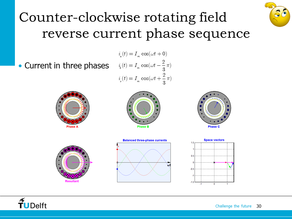
The animation below may also help you understand the rotational magnetic field generated from three phases.

22.4. Number of pole pairs

Now let us study how the number of pole pairs affect the rotational speed of the magnetic field.

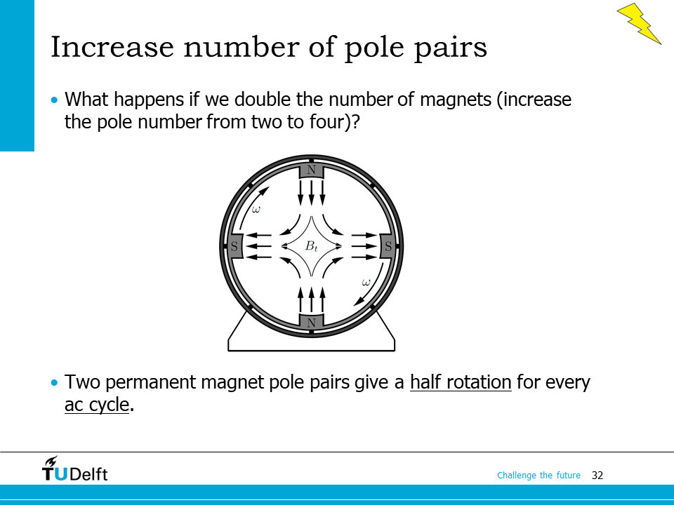
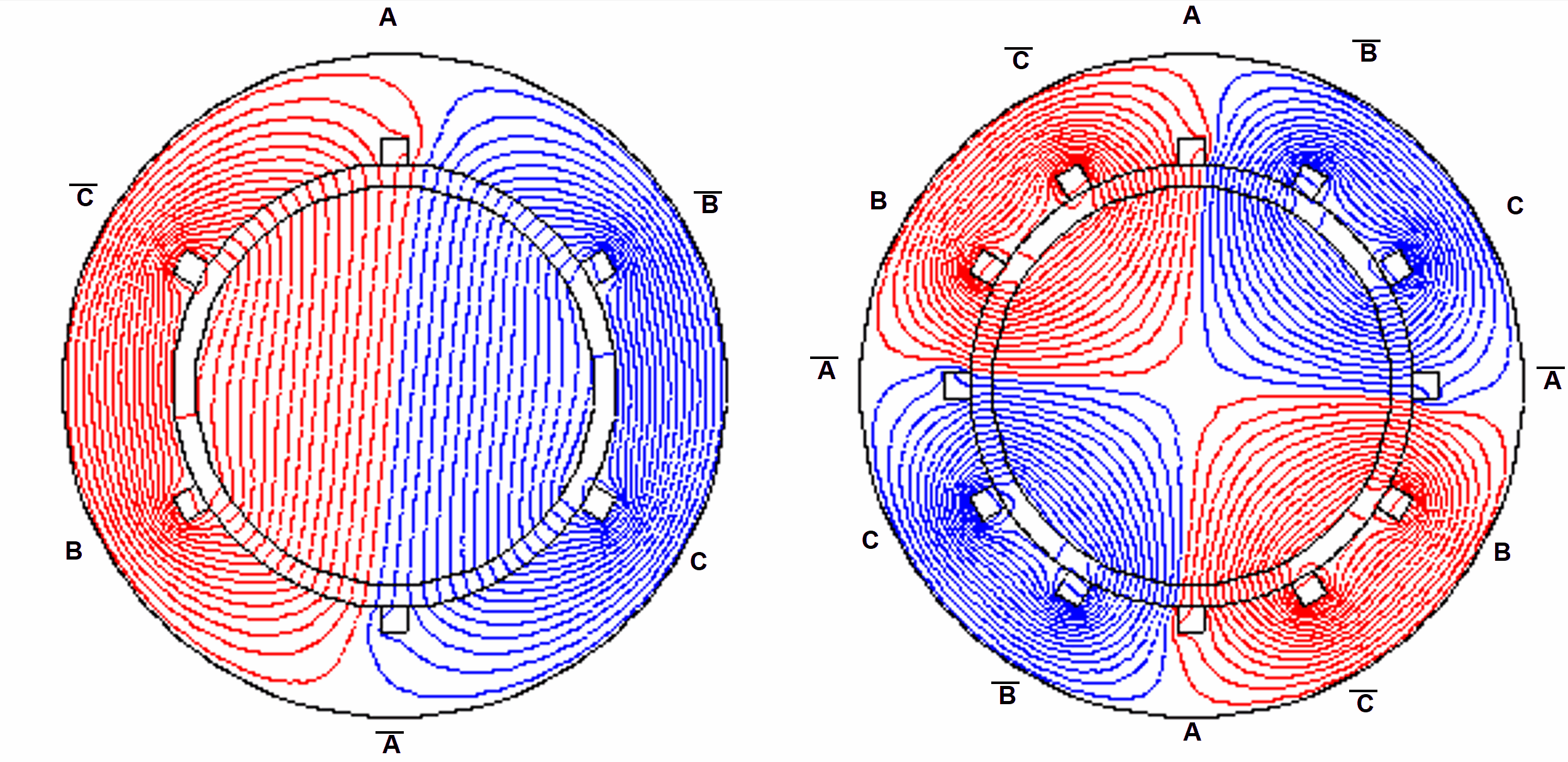
As is illustrated on the slide, if we double the number of pole pairs, when the rotor rotates by one revolution, the changing cycle of the magnetic field we get is also doubled, i.e., if we put a coil on the stator, the frequency of the induced voltage is also doubled.

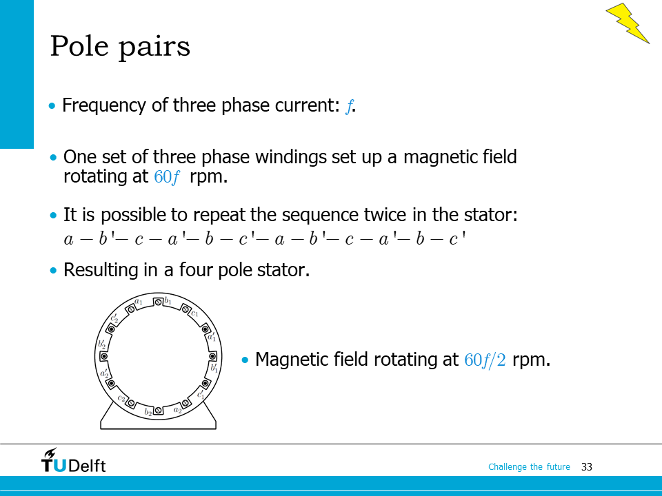
If the three phase stator currents have a frequency of \(f\), with one set of a-b-c winding sequence, we will have a rotational speed of the magnetic field as \(60f\) rpm. However, if we repeat the a-b-c winding sequence twice on the stator to double the number of pole pairs of the generated magnetic field, we will see for the same \(f\), the rotational frequency of the magnetic field is actually reduced to half.

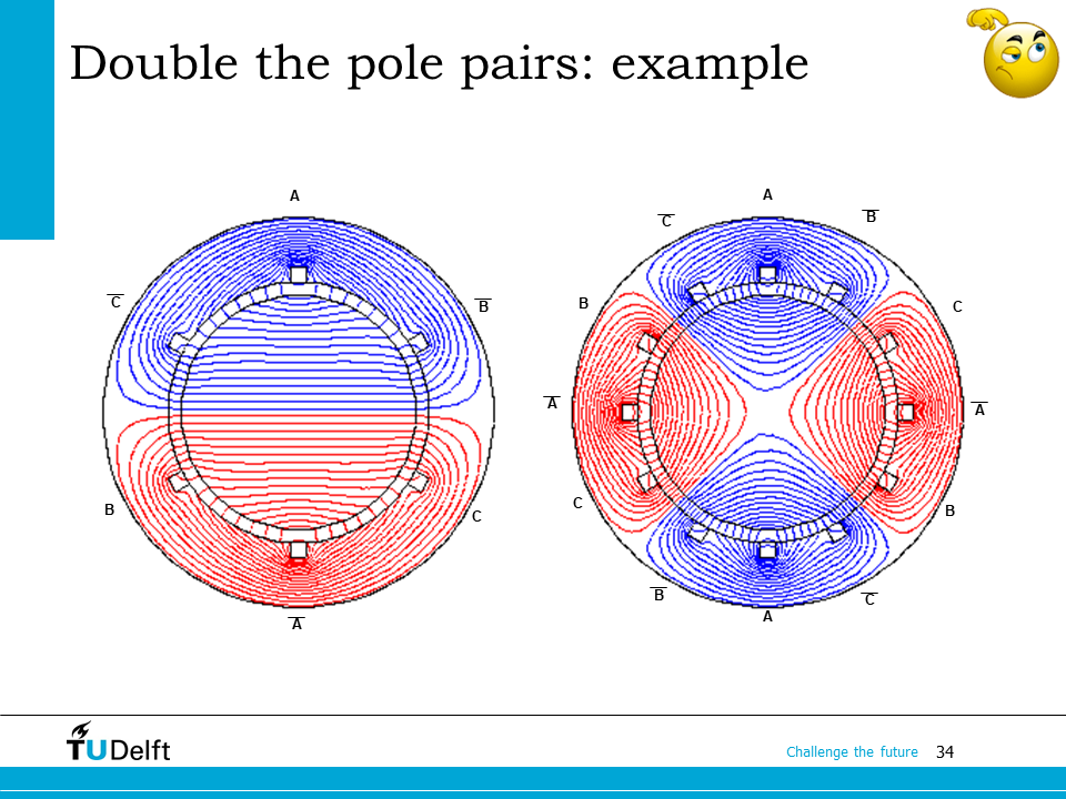
The animation below shows how doubling the magnetic poles can reduce the field rotational speed when the current frequency is kept the same.

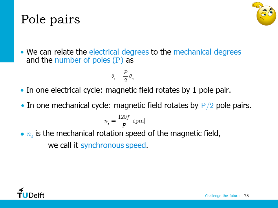
As we can see, it is necessary to relate the electrical quantities to the mechanical quantities. The electrical degrees an electrical waveform travels \(\theta_e\) can be related to the mechanical degree the field travels \(\theta_m\) as

\[ \theta_e = \frac{P}{2}\theta_m. \]

Attention

The capital \(P\) is used to note the number of poles, while the small letter \(p\) is used for number of pole pairs. Therefore \(p = P/2\).

In one electrical cyle, the magnetic field rotates by 1 pole pair. If there are \(P/2\) pole pairs in one mechanical cycle, we know the electrical frequency can be related to the mechanical rotational speed by

\[ n_s = \frac{60f}{P/2} [rpm]. \]

Here \(n_s\) is the mechanical rotational speed of the magnetic field. We define it as the synchronous speed since it is synchronised to the rotation of the magnetic field.

Induced voltage

We have studied how three phase currents can generate a rotational magnetic field. In order to enable the electromechanical energy conversion, we also need to have three phase induced voltages in the three phase windings.

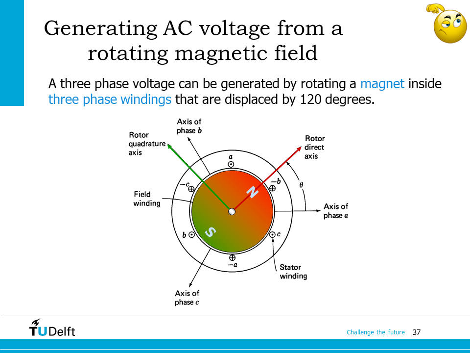
If there are permanent magnets on the rotor, and generate a rotating magnetic field, by putting the three phase windings on the stator side and displace them by 120 degree from each other, we are able to have three induced voltages, and the phase different between them would also be \(\frac{2\pi}{3}\).

In practice, the permanent magnets can also be replaced with a field winding to generate the magnetic field.

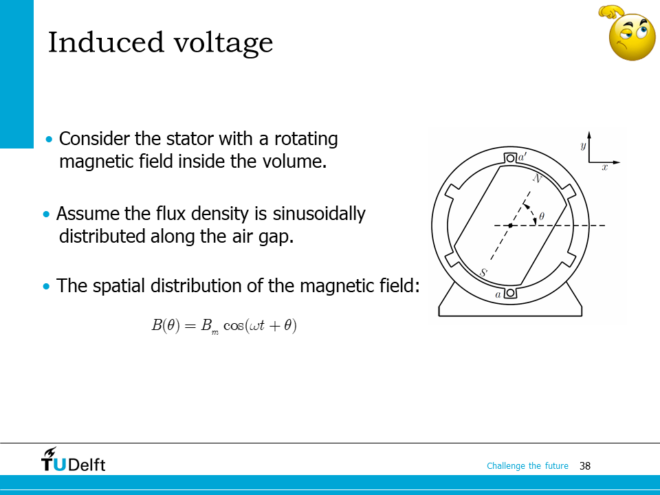
Now let us quantitatively investigate the induced voltage. First, we describe the rotating magnetic field as

\[ B(\theta) = B_m\cos(\omega t+\theta). \]

where \(\theta\) is the spatial angle in the air gap.

For winding \(a\) which is spanning from \(-\pi/2\) to \(\pi/2\), the flux linkage links with phase \(a\) can then be obtained from the integral:

\[\begin{split} \begin{align} \lambda_a &= N\phi_a(\theta) = \int_{-\frac{\pi}{2}}^{\frac{\pi}{2}}B(\theta)lr\mathrm{d}\theta \\ &=N\int_{-\frac{\pi}{2}}^{\frac{\pi}{2}}B(\omega t+\theta)lr\mathrm{d}\theta \\ &= 2NB_mlr\cos(\omega t). \end{align} \end{split}\]

Applying Faraday’s law, the induce voltage is solved as

\[ e_a(t) = -2\omega NB_mlr\sin(\omega t) = E_m\sin(\omega t). \]

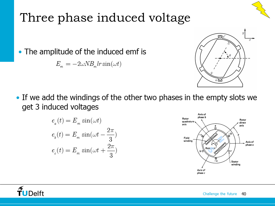
Since the other two phases are displaced from phase \(a\) by 120 degree in space, we can derive that the three phase flux linkages are

\[\begin{split} \begin{align} \lambda_a &= N\phi_a(\theta) = \int_{-\frac{\pi}{2}}^{\frac{\pi}{2}}B(\theta)lr\mathrm{d}\theta \\ \lambda_b &= N\phi_a(\theta) = \int_{-\frac{\pi}{2}+\frac{2\pi}{3}}^{\frac{\pi}{2}+\frac{2\pi}{3}}B(\theta)lr\mathrm{d}\theta \\ \lambda_b &= N\phi_a(\theta) = \int_{-\frac{\pi}{2}-\frac{2\pi}{3}}^{\frac{\pi}{2}-\frac{2\pi}{3}}B(\theta)lr\mathrm{d}\theta \end{align} \end{split}\]

Therefore, the three phase induced voltages are

\[\begin{split} \begin{align} e_a(t) &= E_m\sin(\omega t) \\ e_b(t) &= E_m\sin(\omega t-\frac{2\pi}{3}) \\ e_c(t) &= E_m\sin(\omega t+\frac{2\pi}{3}). \end{align} \end{split}\]

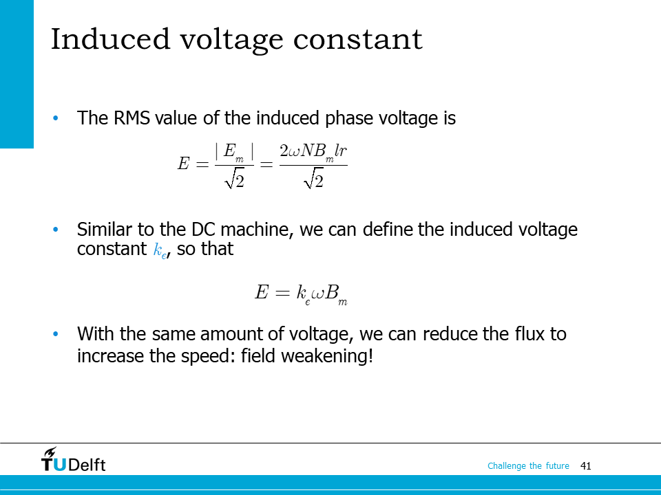
The rms value of the induced phase voltage is then \(E = \frac{|E_m|}{\sqrt{2}} = \sqrt{2}\omega NB_m lr\).

Similar to the DC machine, we can see that the induced voltage is proportional to both the speed and the flux density. Therefore, it is possible to do field weakening to increase the operable speed, so that the induced voltage is within the voltage limit, as we have done in DC drives.