20. DC Machine Performance#
In this lecture we will study the performance of the DC machine in detail. We will start from learning how to read a nameplate of the machine, then move on to various characteristics of the DC machine. After taking the lecture, we should be able to understand different excitation configurations of DC machines, their two operation modes and the power flows in the two operation modes.
20.1. DC Machine recap#
Let us first review what we have learned in the last lecture.
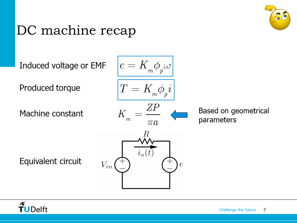
In the last lecture, the machine constant \(K_m\) of the DC machine is introduced, which bridges the electrical equivalent circuit with the electromagnetic torque.
By combining the machine constant, the induced voltage equation, torque equation and the equivalent circuit, we would be able to solve the performance of any DC machines in steady state.
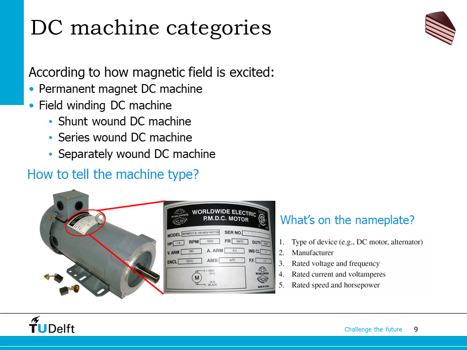
In the last lecture, we briefly mentioned DC machines can be categorised into two categories: field winding DC machine and permanent magnet DC machine, based on how the magnetic field is excited.
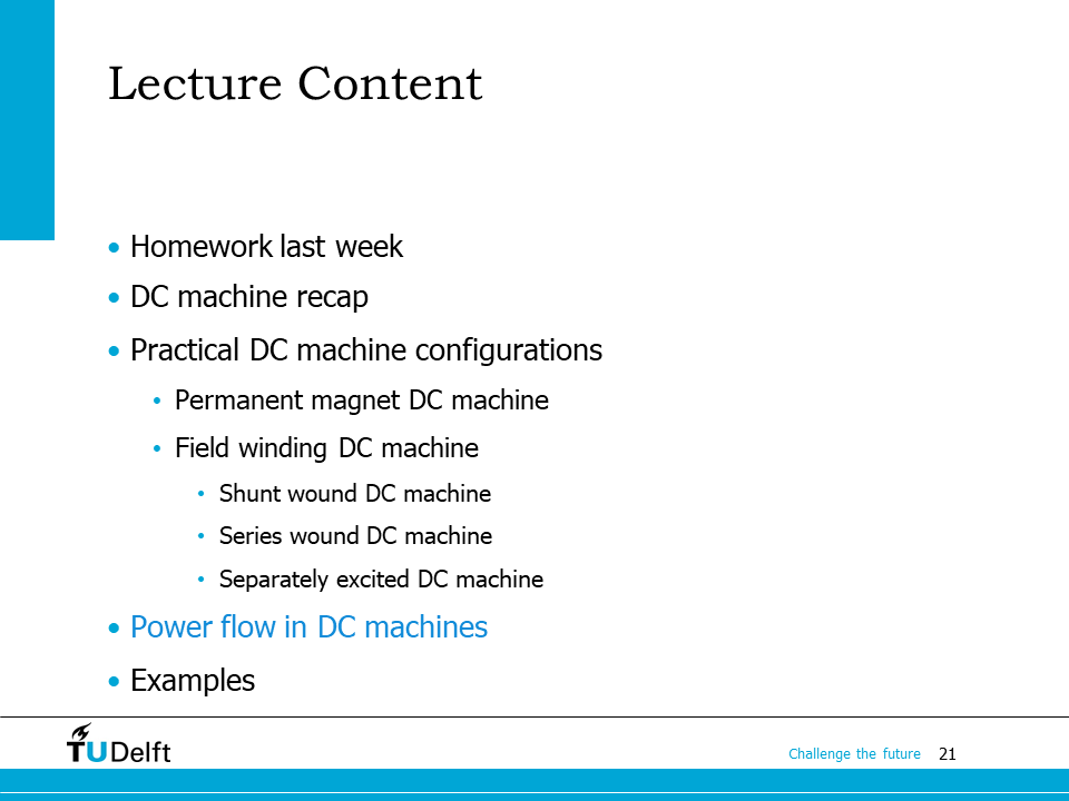
In this lecture we will see depending on how the field winding and the armature winding are connected, the field winding DC machine can be further classified into shunt DC machine, series DC machine, separately excited DC machine and compounded DC machine.
In practice, to tell the type of any electrical machines, we have to check the nameplate attached to the frame of them. On this slide, you can see there is a nameplate attached to the frame of the machine. On the nameplate, you can see it is a “P.M.D.C MOTOR”, or a permanent magnet DC motor. Below the type of motor, you can see the rated parameters of it, as shown below.
Parameters |
Values |
|---|---|
Rated power |
1.5 hp |
Rated armature voltage |
180 V |
Rated armature current |
8 A |
Rated speed |
1800 rpm |
Enclosure type |
TEFC (totally enclosed, fan cooled) |
Duty |
Continuous |
Note
\(\mathrm{hp}\), or horse-power is a unit of power, which is commonly used in the US.
20.2. Permanent Magnet DC Machine#
The permanent magnet DC machine performance is first studied since the construction is the simplest.
Permanent magnets are hard magnetic materials, which means they have large magnetic hysteresis loop. Once they are magnetised, it is much more difficult to make them lose magnetisation by applying external field. On the other hand, the ferromagnetic material used to make magnetic cores for stators and rotors, should have hysteresis loops as small as possible, to reduce hysteresis loops.
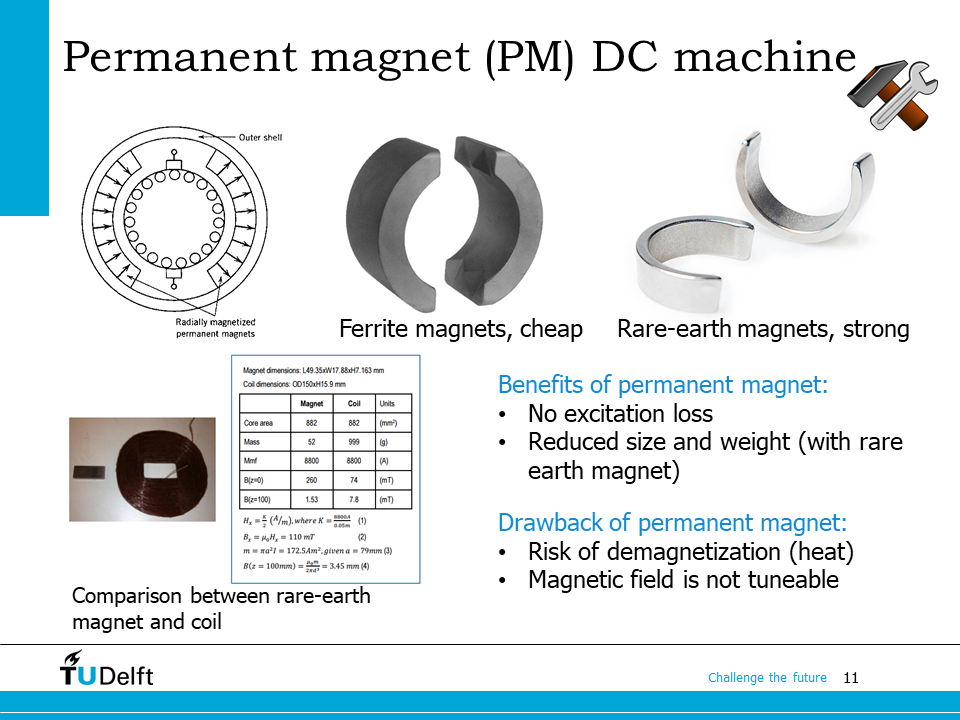
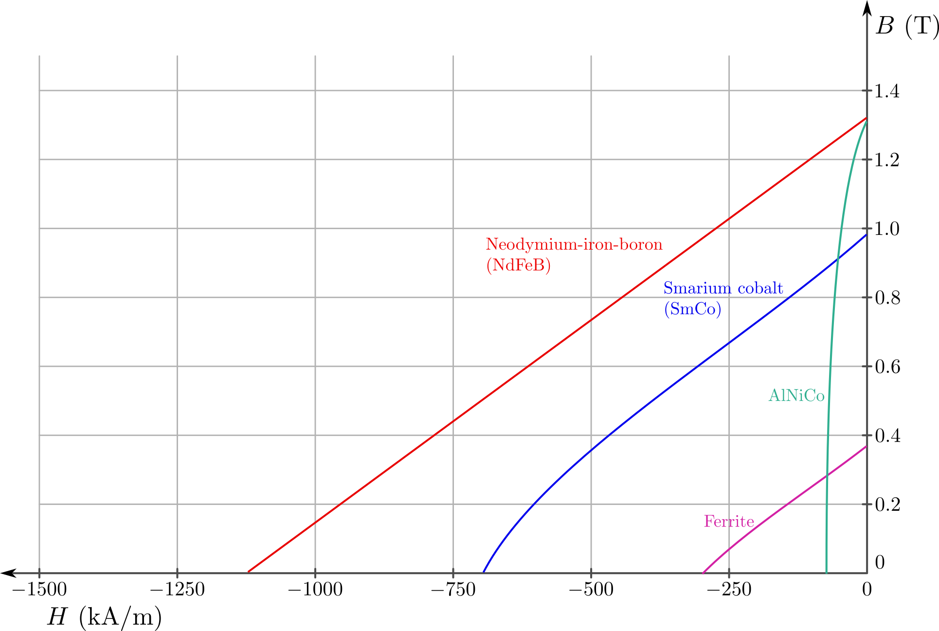
The permanent magnets for the poles of a permanent magnet DC (PMDC) motor operate in the 2nd quadrature of its hysteresis loop. The image below shows the BH curve of mainstream permanent magnets used in electrical machines. The cross point of the BH curve with the y-axis is the residual flux density \(B_r\), while the cross point with the x-axis is called the coercive magnetising intensity \(H_c\). A permanent magnet (PM) is considered to be stronger if its \(B_r\) and \(H_c\) have larger values simultaneously. The strongest permanent magnets at the moment are rare-earth magnets, including two types: neodymium magnets (NdFeB) and samarium–cobalt magnets. They are commonly used in high end motors for electric vehicles and servo systems. Permanent ferrite magnets (hard ferrites) are less strong, but are much cheaper. You may find them used in domestic applications such as washing machines and toys.
A PM machine has many advantages, such it does not need conductors to excite the magnetic field, hence there are no field circuit copper losses. The machine can be made much smaller. As shown in the left figure on the slide, to generate the same field level, the size and weight of the required rare earth PM is much smaller than that of copper wires.
The PM machines also have disadvantages, e.g. the magnetic field is not tuneable, and it can be irreversibly demagnetised by high temperature caused by losses when overloaded.
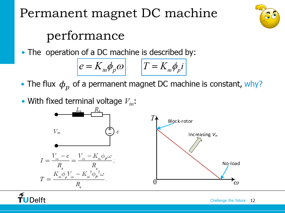
The flux of a PMDC machine is fixed, because the field excited from the permanent magnets are not tuneable. Therefore, based on the induced voltage equation, torque equation and the equivalent circuit, we are able to derive the armature current and the torque:
The torque-speed characteristic of the PMDC machine can be plotted from the equation above. As we can see, it is a straight line, and as the armature terminal voltage \(V_{in}\) increases, the characteristic line moves up, but the slope remains the same, which is \(-K_m^2\phi_P^2/R_a\).
From the characteristic above we can see, to control of the speed of a PMDC machine, we can only vary the armature voltage or the armature resistance.
The cross point of the \(T-\omega\) characteristic line with the \(T\) axis is called the block-rotor torque, while that with the \(\omega\) axis is called the no-load speed.
20.3. Field winding DC Machine#
The field winding DC machine is more complicated since it has two windings: the field winding and the armature winding, which enables various connection configurations.
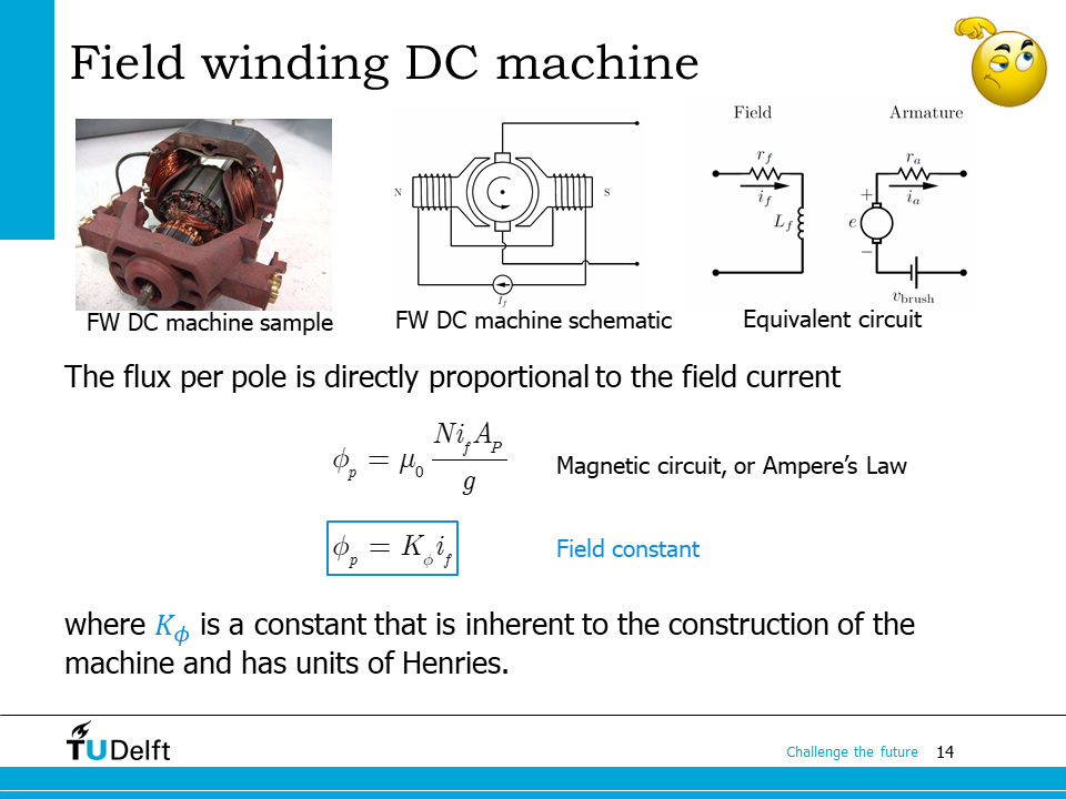
Supposing the number of turns on one pole is \(N\), the air-gap length is \(g\), and the field current is \(i_f\), we can derive from Ampere’s law that the flux density under the pole is
The flux per pole is
Similar to the definition of the machine constant, we can collect all the geometrical parameters and \(\mu_0\) in the above equation, so
where \(K_{\phi}\) is defined as the field constant. It has a unit of \([\mathrm{Vs/A}]\), \([\mathrm{Wb/A}]\) or \(\mathrm{H}\), which is the same as the unit for the inductance.
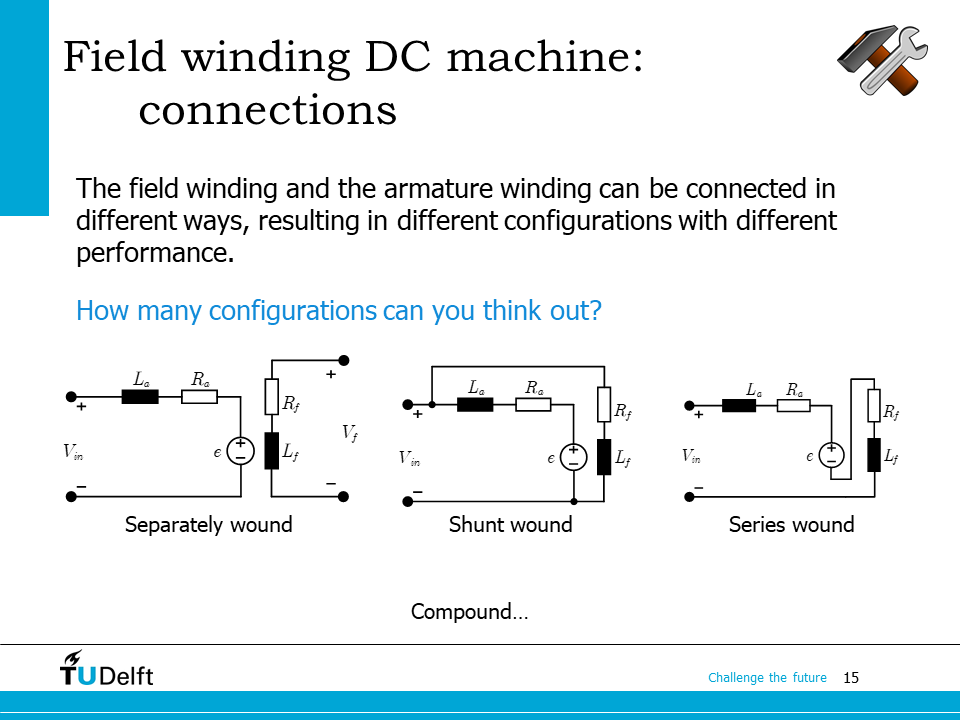
Depending on how the field winding and the armature winding are connected, we can divide the wound field DC machine into different types. On the slide you can see
- Separately DC machine#
The field circuit and the armature circuit are supplied from two separate supplies.
- Shunt DC machine#
The field circuit and the armature circuit are connected in parallel and supplied from the same supply.
- Series DC machine#
The field winding is connected in series with the armature circuit.
There is also the compounded DC machine, where the motor has both a shunt and a series field circuit, which is out of the scope of the course.
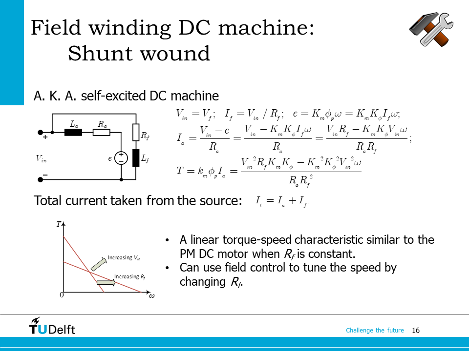
We first study the characteristic of a shunt DC machine. First we solve the field current from the field circuit:
The flux per pole is \(\phi_P = K_\phi I_f = K_\phi V_{in}/R_f\). Then the induced voltage is
The armature current is solved from the armature circuit:
The torque is then calculated as
From the equation above, we can see the torque-speed characteristic of the shunt DC machine is still a straight line with a negative slope. If we increase the terminal voltage \(V_{in}\), the block rotor torque increases and the \(T-\omega\) line becomes steeper. If we increase \(R_f\), the block rotor torque reduces, and the \(T-\omega\) line becomes less steep. The same applies to \(R_a\). Therefore, we are able to control the speed of the shunt DC machine by varying \(V_{in}\), or the resistances connected in series with the two windings.
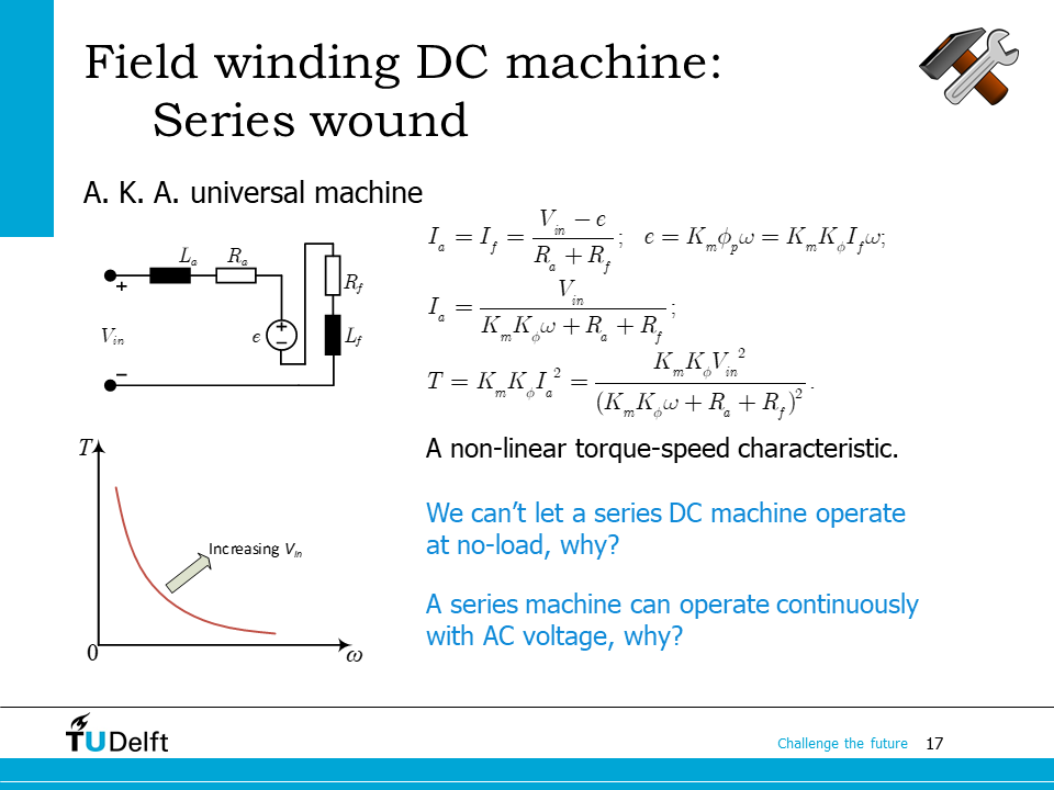
In a series DC machine, the armature current and the field current are the same:
where the induced voltage \(e = K_m\phi_P\omega = K_mK_\phi I_f\omega\).
From the above two equations, the current is solved
The torque is
which result in a sharply drooping non-linear torque-speed characteristic. As plotted on the slide, when the torque on applied on the machine goes to zero, its speed goes to infinity. The zero torque case never happens in practice because there is always mechanical loss and core loss to overcome. However, if there is no other external load connected, it can turn at an extremely high speed, so high that it can damage itself. Therefore, we should never unload a series DC machine completely or connect the load to it via a mechanism which can break, e.g., via a belt.
The series machine has very high block-rotor torque, which makes it suitable for applications where high torque is required at low speeds, e.g., handheld tools, and starter motor for fuel engines.
Another appealing feature of the series DC machine is it is able to operate with single phase AC supply. As we can see from the equivalent circuit, as \(V_{in}\) reverses its polarity, both \(I_f\) and \(I_a\) change their polarities, which result in a uni-directional torque. Therefore, it is also called a universal motor. To change the direction of the torque, we can just swapping the polarity of either field or the armature winding.
Because of the high torque and AC operable features, the series machine used to be extensively used as tractor motors in locomotives. Nowadays they have been replaced with AC induction or synchronous machines fed by power electronics converters, mainly because of the availability of reliable high power semiconductors since 1960s.
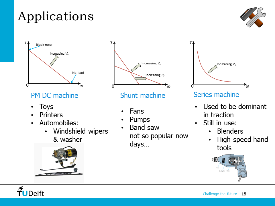
Here it lists the suitable applications for the three types of DC machines based on its torque-speed characteristics.
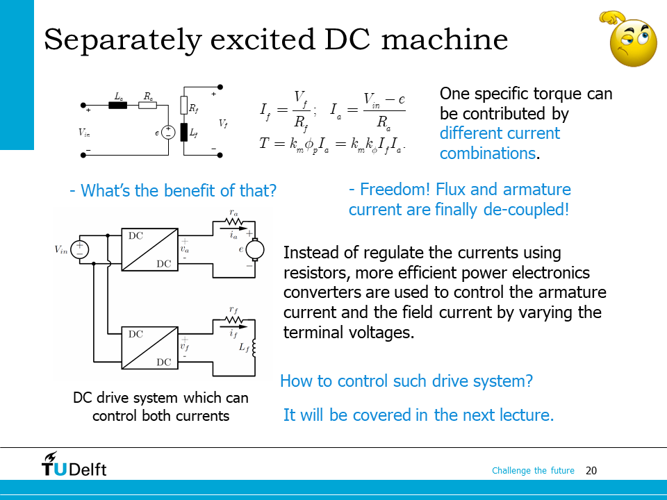
The last type of DC machine we study in this lecture is the separately excited DC machine. The armature winding and the field winding are separately supplied with two separate power supplies. Therefore, \(I_f\) and \(I_\phi\) are independent from each other. There are multiple \(I_f\) and \(I_\phi\) combinations to contribute to one specific torque, which provides the freedom to control the flux and the armature current in a decoupled way.
As we can see on the left hand side, the field circuit and armature circuit can be supplied by two separate DC-DC converters. Thus \(I_f\) and \(I_\phi\) can be regulated in a more efficient way compared to the resistor based method.
In the next lecture, we will study how to use DC converters to make a modern DC drive system, and how the DC drive system performs.
20.4. Power flow in DC machine#
The last topic for today is the power flow and efficiency calculation of DC machines.
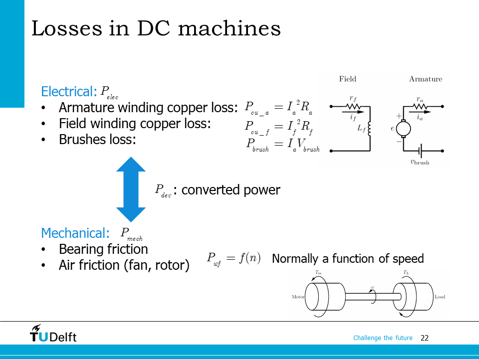
There are also losses happening during the electromechanical energy conversion process. On the electrical side, the armature winding has copper loss, which is caused by the winding resistance.
Similarly, the field winding also has copper loss because of its resistance
There is also brush voltage drop \(V_{brush}\) when the armature current is flowing between the brush and the commutator, it creates a loss of
On the mechanical side, the losses are brought by the mechanical friction in the bearings, and air dragging on the rotor and the cooling fan when they rotates. These mechanical losses are normally a function of speed, and represented as \(P_{wf}\) in this course.
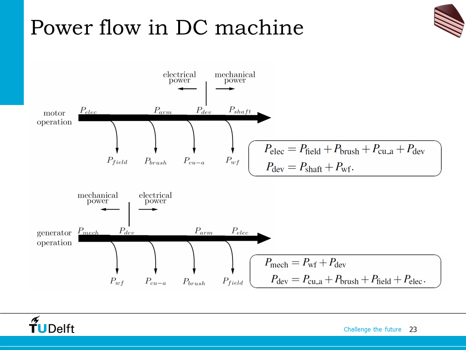
Depending on the direction of power flow, we can divide the electrical machine operation mode to the motor operation and generator operation. In both operations, we define the part of power which really participates in the electromechanical energy conversion as developed power, or \(P_{dev}\).
In the motor operation, the machine takes electrical power \(P_{elec}\) as input, which consists of the electrical losses and the developed power. Then the developed power is converted to the mechanical power, which consists of the mechanical loss \(P_{wf}\), and the mechanical power delivered to the shaft \(P_{shaft}\). Mathematically, the energy conversion process can be expressed as
The power efficiency in the motor operation is then
The power flow in the generator operation is reversed. The input power is the mechanical power \(P_{mech}\) applied to the shaft, which consists of the mechanical loss \(P_{wf}\) and the developed power \(P_{dev}\). The developed power \(P_{dev}\) is then converted to the electrical power, which consists of the electrical losses, and the output electrical power to the electrical terminal \(P_{elec}\). Mathematically, we have
The power efficiency in the generator operation is then
20.5. Examples#
In the end of the lecture, there are some examples to practice the performance calculation of DC machines.
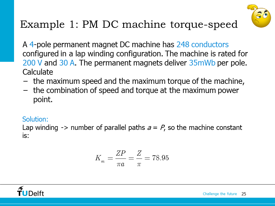
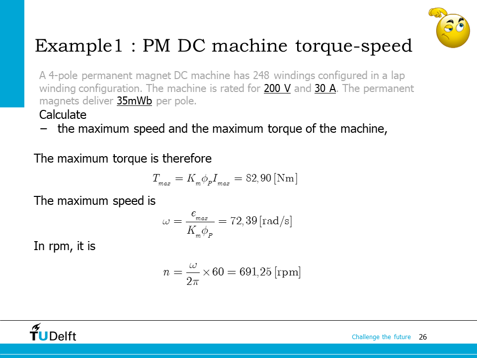
Example 1 is about the torque-speed characteristic of a PM DC machine.
Please first try to work it out yourself, and click the hidden content below to check your answer.
Click here for solution
Show code cell source
import numpy as np
P = 4 # number of poles
Z = 248 # number of conductors
Vrate = 200 # rated voltage
Irate = 30 # rated current
phi_P = 0.035 # flux per pole
R_a = 0.02 # armature resistance
# first we calculate the machine constant
# Since it has a lap winding, the number of parallel paths a = P
a = P
K_m = Z*P/np.pi/a
# 1. maximum speed and maximum torque
# maximum speed happens when the torque is zero (no-load speed)
# or cross point between T-n curve and the n axis, where Ia = 0, T = 0
omega_max = Vrate/K_m/phi_P
n_max = omega_max*60/(2*np.pi)
# maximum torque happens when the current is the maximum (rated current)
T_max = K_m*phi_P*Irate
print(f'1. The maximum speed is n_max = {n_max:.3f} rpm.')
print(f'The maximum torque is T_max = {T_max:.3f} Nm.\n')
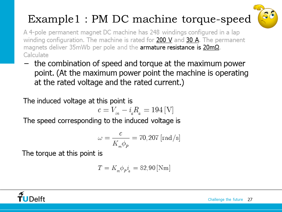
# 2. maximum power point happens when the voltage and current are both at rated value
# induced voltage
e = Vrate - Irate*R_a
# speed
omega = e/K_m/phi_P
# convert to rpm
n = omega/(np.pi*2)*60
# torque
T = K_m*phi_P*Irate
print(f'2. The speed at maximum power poitn is n = {n:.3f} rpm, or omega = {omega:.3f} rad/s.')
print(f'The maximum torque is T = {T:.3f} Nm.')
1. The maximum speed is n_max = 691.244 rpm.
The maximum torque is T_max = 82.888 Nm.

2. The speed at maximum power poitn is n = 689.171 rpm, or omega = 72.170 rad/s.
The maximum torque is T = 82.888 Nm.
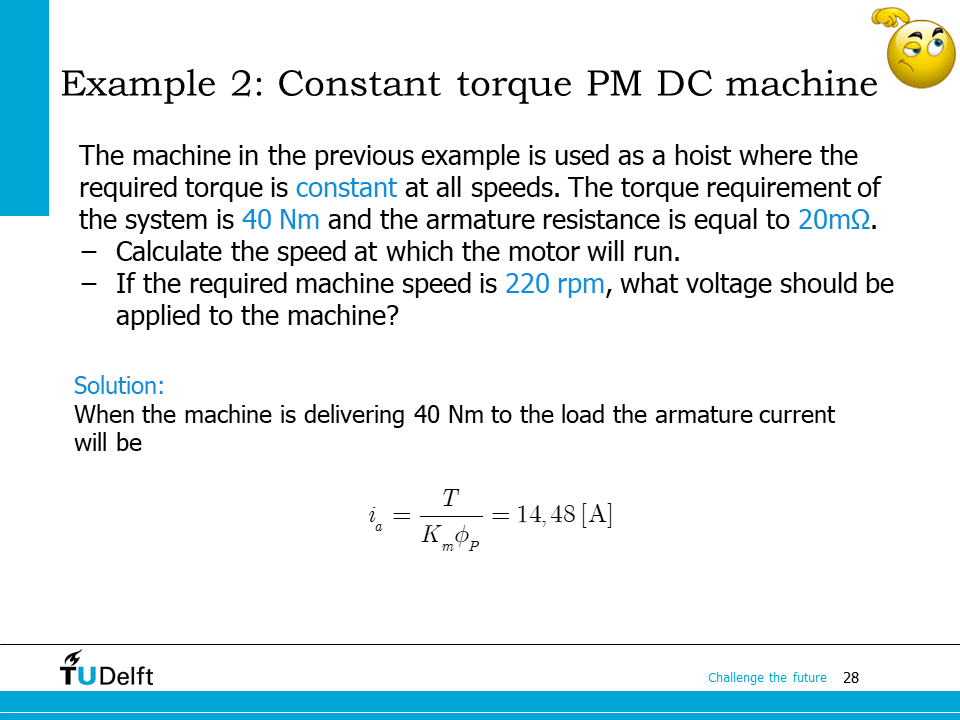
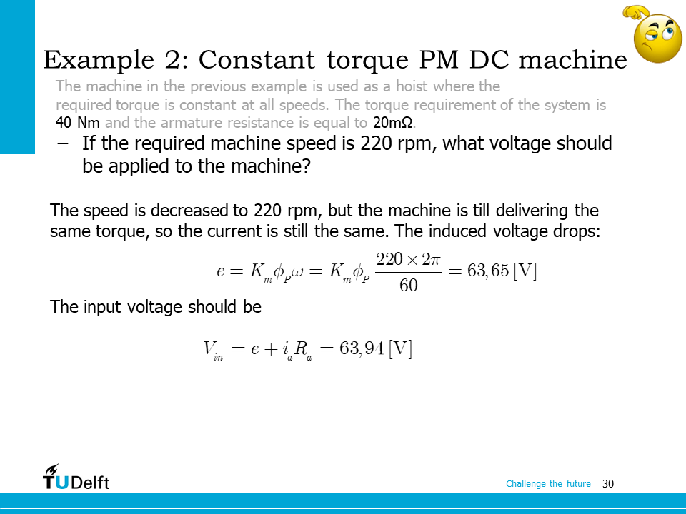
The second example is more complicated. Please try to solve it yourself, and click the hidden content below to check your answer.
Click here for solution
Show code cell source
import numpy as np
T = 40.0 # required torque
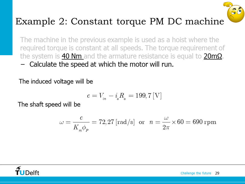
# 1. speed at 40 Nm
# to get the speed, we need to know the induced voltage
# which is obtained from the armature current and the Kirchhoff Law
Ia = T/(K_m*phi_P)
e = Vrate - Ia*R_a
omega = e/(K_m*phi_P)
n = omega*60/(2*np.pi)
# 2. voltage at 220 rpm
# similar to the previous question, we first get induced voltage
e = K_m*phi_P*(220.0/60*2*np.pi) # 220 rpm
# then get the input voltage from Kirchhoff's Law
Vin = e+R_a*Ia
print(f'1. The speed is n = {n:.3f} rpm.')
print(f'2. The input voltage is Vin = {Vin:.3f} V.')
1. The speed is n = 690.243 rpm.
2. The input voltage is Vin = 63.943 V.